Algorithmic approaches
Introduction
Here we show how you can estimate crop calendars with a simple algorithm
based on rainfall. This approach, and similar approaches, should work
particularly well in regions with a short and well-defined growing
season, but it can be used under different conditions as well. Note that
we only use rainfall, and ignore temperature. This algorithm was
developed for maize in Sub-Saharan Africa, and perhaps seasonal
variation in temperature can be ignored there, but at high latitudes it
must certainly be included. You can expand the algorithm used here to
include temperature; or have a look at the ecolim approach, that
uses both rainfal and temperature, and is described in the next
chapter.
Chapter requirements
We use R packages agro and geodata. See these
installation instructions.
Function
We use the function agro::plant_harvest. See
?agro::plant_harvest. Here we show the source code of the function,
including the comments that may help you understand what the function
does.
plant_harvest <- function(x, min_prec=30, max_prec=90, max_len=5) {
## check input
# must have 12 values (months)
    stopifnot(length(x) == 12)
# cannot have any NAs
    if (any(is.na(x))) return (matrix(NA, nrow=12, ncol=2))
# max_len is the number of months
    stopifnot(max_len > 0 & max_len <= 12)
# min precipitation threshold below max threshold
    stopifnot(min_prec < max_prec)
## compute threshold
# median of the rainfall
    med <- stats::median(x)
# median clamped between min_prec and max_prec
    prec_threshold <- min(max_prec, max(min_prec, med))
# make a time series of 24 months, from July to July, to make it easier
# to do 'circular' computation across the year boundary. That is, we
# cannot ignore that (January comes after December)
    x24 <- c(x[7:12], x, x[1:6])
# which months are above the threshold?
    above_th <- x24 >= prec_threshold
# cumulate successive months above the threshold
    y <- cumsum(above_th)
# remove months below the threshold and reset
# the beginning of a sequence to 1
# (perhaps the most obscure step)
    wet <- (y - cummax(y * !above_th))
# go back to a single 12 months (Jan to Dec) year
    wet <- wet[7:18]
# set up output
    planting <- harvest <- rep(0, 12)
# find the length of the growing season
    m <- min(max_len, max(wet))
# growing season must be at least 3 months
    if (m > 2) {
    # harvest months
        harvest[wet >= m] <- 1
    # planting months
        p <- which(wet >= m) - m + 1
    # 1 month before January -> December
        p[p < 1] <- 12 + p[p < 1]
        planting[p] <- 1
    }
    return( cbind(planting=planting, harvest=harvest) )
}
First try it
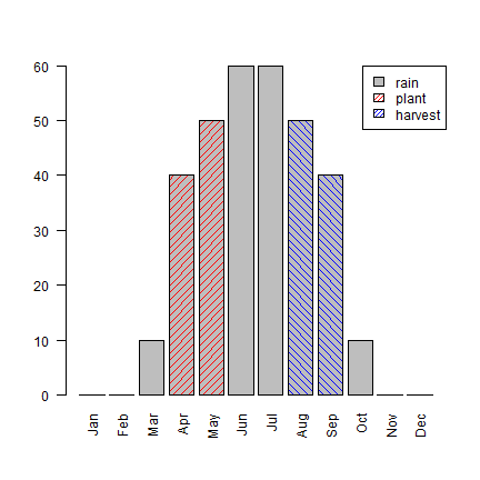
It is often useful to try an algorithm on simple contrived data, before using it on real-world data. Here we look at four imaginary locations. First a location with a single rainy season.
Single season
rain <- c(0,0,10,40,50,60,60,50,40,10,0,0)
agro::plant_harvest(rain)
##       planting harvest
##  [1,]        0       0
##  [2,]        0       0
##  [3,]        0       0
##  [4,]        1       0
##  [5,]        1       0
##  [6,]        0       0
##  [7,]        0       0
##  [8,]        0       1
##  [9,]        0       1
## [10,]        0       0
## [11,]        0       0
## [12,]        0       0
Here are two helper functions, both to display the results in a nicer way.
The below function makes printed output more readable.
printSeason <- function(rain) {
    x <- agro::plant_harvest(rain)
    rownames(x) <- month.abb
    t(x)
}
Let’s try it:
printSeason(rain)
##          Jan Feb Mar Apr May Jun Jul Aug Sep Oct Nov Dec
## planting   0   0   0   1   1   0   0   0   0   0   0   0
## harvest    0   0   0   0   0   0   0   1   1   0   0   0
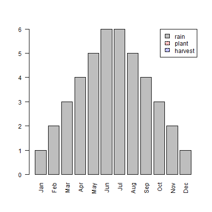
We can also make a barplot
plotSeason <- function(rain) {
    x <- agro::plant_harvest(rain)
    barplot(rain, names.arg=month.abb, las=2)
    barplot(x[,1]*rain, add=T, col="red", axes=FALSE, density=15)
    barplot(x[,2]*rain, add=T, col="blue", axes=FALSE, density=15, angle=315)
    legend("topright", c("rain", "plant", "harvest"), fill=c("gray", "red", "blue"), density=c(-1,25,25))
}
Use the function with the rain defined above.
plotSeason(rain)
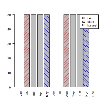
Bi-modal season
Now a location with a bi-modal rainy season
rain <- c(0,rep(50,4), 0, 0, rep(50,4), 0)
rain
##  [1]  0 50 50 50 50  0  0 50 50 50 50  0
printSeason(rain)
##          Jan Feb Mar Apr May Jun Jul Aug Sep Oct Nov Dec
## planting   0   1   0   0   0   0   0   1   0   0   0   0
## harvest    0   0   0   0   1   0   0   0   0   0   1   0
plotSeason(rain)
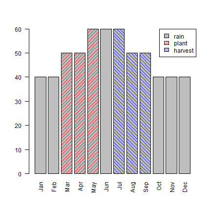
Year-round rain
In a place where rains year-round you may planting and harvesting every month of the year.
rain <- c(4,4,5,5,6,6,6,5,5,4,4,4) * 10
rain
##  [1] 40 40 50 50 60 60 60 50 50 40 40 40
printSeason(rain)
##          Jan Feb Mar Apr May Jun Jul Aug Sep Oct Nov Dec
## planting   0   0   1   1   1   0   0   0   0   0   0   0
## harvest    0   0   0   0   0   0   1   1   1   0   0   0
plotSeason(rain)
Arid conditions
When it is too dry to grow much, you can never plant or harvest.
rain <- c(1:6, 6:1)
printSeason(rain)
##          Jan Feb Mar Apr May Jun Jul Aug Sep Oct Nov Dec
## planting   0   0   0   0   0   0   0   0   0   0   0   0
## harvest    0   0   0   0   0   0   0   0   0   0   0   0
plotSeason(rain)
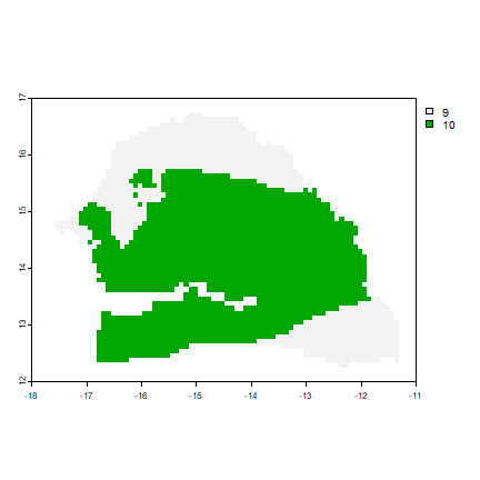
Apply it
Now, let’s apply this to Senegal. First we get WorldClim data.
library(geodata)
rain <- geodata::worldclim_country("Senegal", var="prec", path=".")
adm <- geodata::gadm("Senegal", level=1, path=".")
rain <- mask(rain, adm)
names(rain) <- month.abb
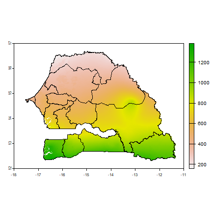
Annual rainfall
plot(sum(rain))
lines(adm)
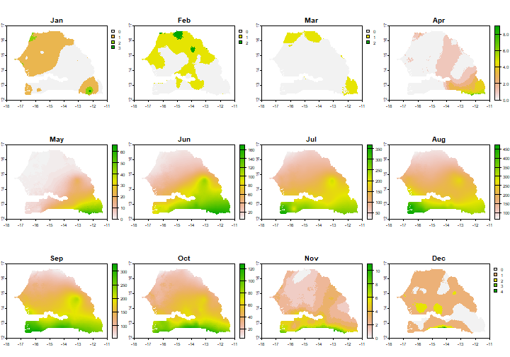
Monthly rainfall
plot(rain)
Aggregate the data a bit to speed up computations
arain <- aggregate(rain, 10, mean, na.rm=TRUE)
Now “apply” the function “plant_harvest” to SpatRaster “rain”
x <- app(arain, agro::plant_harvest)
x
## class       : SpatRaster
## dimensions  : 60, 84, 24  (nrow, ncol, nlyr)
## resolution  : 0.08333333, 0.08333333  (x, y)
## extent      : -18, -11, 12, 17  (xmin, xmax, ymin, ymax)
## coord. ref. : lon/lat WGS 84 (EPSG:4326)
## source(s)   : memory
## names       : lyr.1, lyr.2, lyr.3, lyr.4, lyr.5, lyr.6, ...
## min values  :     0,     0,     0,     0,     0,     0, ...
## max values  :     0,     0,     0,     0,     1,     1, ...
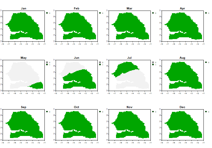
Output x has 24 layers, matching the output of plant_harvest (12 for
planting, and 12 for harvest). Let’s separate them.
plant <- x[[1:12]]
names(plant) <- month.abb
harv <- x[[13:24]]
names(harv) <- month.abb
And have a look
plot(plant)
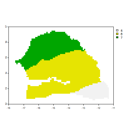
First month of planting
plantna <- classify(plant, cbind(0, NA))
p <- which.max(plantna)
plot(p)
First month of harvest (note that which works here because the
harvest is in the same calendar-year as planting.
harvna <- classify(harv, cbind(0, NA))
h <- which.max(harvna)
plot(h)