Crop calendars
Introduction
To model regional crop growth we need to know when crops are actually grown. When are the crops planted, when are they harvested? Crop calendars describe planting and harvesting times. There have been some efforts to compile them into spatial databases.
In this chapter, we discuss three data sources on global crop calendars. “Sacks” has calendars for 19 crops. Whereas “MIRCA2000” has calendars for 26 irrigated and rainfed crops. Finally a third dataset “RiceAtlas” has global calendars for rice.
Note that there is another section on estimating crop calendars, in which we compare results with these databases and discuss what approach might be best to use.
Chapter requirements
We use R packages terra and geodata.
Sacks data
We first have a look at the Sacks et al. data. Global crop
calendars.
The can be downloaded with the geodata package.
library(geodata)
geodata::crop_calendar_sacks(path=".")
## Choose one of:
##  [1] "barley (winter)"       "barley (spring)"       "cassava"
##  [4] "cotton"                "groundnut"             "maize (main season)"
##  [7] "maize (2nd season)"    "millet"                "oat (winter)"
## [10] "oat (spring)"          "potato"                "pulses"
## [13] "rapeseed"              "rice (main season)"    "rice (2nd season)"
## [16] "rye"                   "sorghum (main season)" "sorghum (2nd season)"
## [19] "soybean"               "sugarbeet"             "sunflower"
## [22] "sweetpotato"           "wheat (winter)"        "wheat (spring)"
## [25] "yam"
There are 25 choices, for 20 crops, as some are divided into two groups (winter / spring) or (main / 2nd season). We choose “Maize (main season)”
Maize, main season
r <- geodata::crop_calendar_sacks("maize (main season)", path=".")
r
## class       : SpatRaster
## dimensions  : 1800, 4320, 6  (nrow, ncol, nlyr)
## resolution  : 0.08333333, 0.08333333  (x, y)
## extent      : -180, 180, -60, 90  (xmin, xmax, ymin, ymax)
## coord. ref. : lon/lat WGS 84 (EPSG:4326)
## source      : Maize.crop.calendar.tif
## names       : plant.start, plant, plant.end, harve~start, harvest, harvest.end
## min values  :          10,   0.5,        31,           1,     0.5,          31
## max values  :         349, 357.5,       365,         335,   363.5,         365
There are 13 variables in this dataset for each crop.
names(r)
## [1] "plant.start"   "plant"         "plant.end"     "harvest.start"
## [5] "harvest"       "harvest.end"
Note that there is “harvest”, “harvest.start”, “harvest.end”, and “harvest.range”, and that these “harvest.*” variables are also avaiable for planting (“plant.start”, etc).
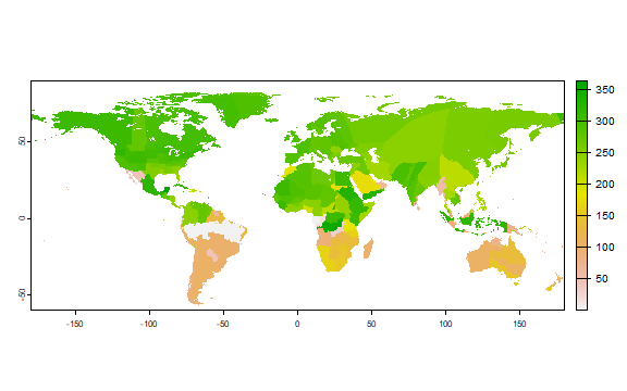
Here is a plot “harvest”, that is, the expected average day of harvest of maize in its main growing season.
plot(r[["harvest"]])
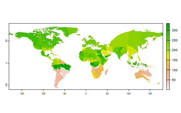
But harvesting is not all done on one day. It is estimated to start on
harvest.start.
plot(r["harvest.start"])
And end on harvest.end.
plot(r["harvest.end"])
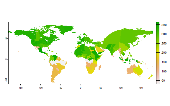
“harvest.range” is the difference between “harvest.start” and “harvest.end”.
grep("plant", names(r), value=TRUE)
## [1] "plant.start" "plant"       "plant.end"
There are some more variables: “harvested.area” has the crop area in ha, and “harvested.area.fraction” has it as a fraction of the grid cell. We do not discuss the crop area data here, as that is the topic of another chapter. Variable “political.level” shows at what level of administrative boundaries data were available to create the planting and harvesting estimates. “index” is just an internal id that is not very relevant to end users.
Maize, second season
Now let’s look at the second maize season
r2 <- geodata::crop_calendar_sacks("Maize (2nd season)", path=".")
r2
## class       : SpatRaster
## dimensions  : 1800, 4320, 6  (nrow, ncol, nlyr)
## resolution  : 0.08333333, 0.08333333  (x, y)
## extent      : -180, 180, -60, 90  (xmin, xmax, ymin, ymax)
## coord. ref. : lon/lat WGS 84 (EPSG:4326)
## source      : Maize.2.crop.calendar.tif
## names       : plant.start, plant, plant.end, harve~start, harvest, harvest.end
## min values  :           1,  29.5,        31,           1,     0.5,          31
## max values  :         305, 350.5,       365,         335,   364.5,         365
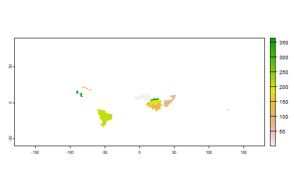
The harvest date for the second season
plot(r2[["harvest"]])
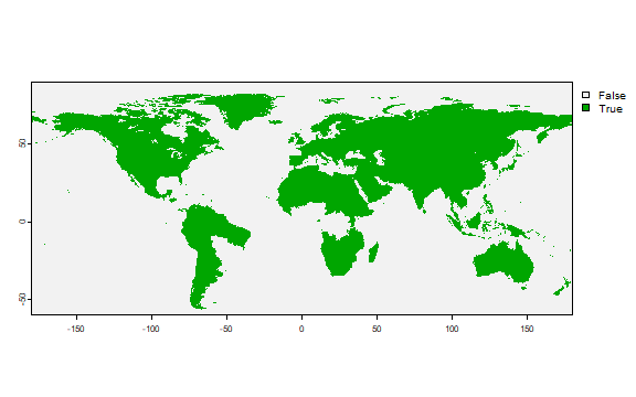
A map showing where there are two seasons. We use the !is.na method.
This works, because anywhere where there is a season, the values are not
NA.
h1 <- r[["harvest"]]
h2 <- r2[["harvest"]]
h12 <- !is.na(h1) + !is.na(h2)
plot(h12)
Here is another way in which you can compute this
x <- c(h1 > 0, h2 > 0)
h12b <- sum(x, na.rm=TRUE)
Rice Atlas
Here is a data source with global rice crop calendars.
#rice <- geodata::crop_calendar_rice()