Spatial QUEFTS
Sebastian Palmas and Robert Hijmans
Introduction
In this chapter we show how to run QUEFTS with spatial data to make predictions. See the previous chapter for a description of the model itself.
Chapter requirements
We use the R packages Rquefts, terra and reagro. See
these instructions about installing these
packages.
Soil data
We use soil raster data for Tanzania from SoilGrids. We changed the pH values from the original data source by dividing them by 10 to get the correct numbers.
library(agrodata)
## Loading required package: terra
## terra 1.7.36
library(terra)
SOC <- reagro_data("TZA_ORC")
Kex <- reagro_data("TZA_EXK")
pH <- reagro_data("TZA_PH")
Need to fix this, there is P data in soilgrids:
“There is no P olsen raster in soilgrids, in the code below we create a constant P Olsen layer by using the soilC layer as a template and assigning all cells a value of 15.”
From these chemical soil properties, we can use QUEFTS to compute the soil nutrient supply.
library(Rquefts)
## Warning: package 'Rquefts' was built under R version 4.3.1
supply <- rast(pH, nlyr=3)
values(supply) <- nutSupply1(pH, SOC, Kex, Polsen=15)
supply
## class       : SpatRaster
## dimensions  : 1191, 1210, 3  (nrow, ncol, nlyr)
## resolution  : 1000, 1000  (x, y)
## extent      : 1037375, 2247375, -1841875, -650875  (xmin, xmax, ymin, ymax)
## coord. ref. : +proj=laea +lat_0=5 +lon_0=20 +x_0=0 +y_0=0 +datum=WGS84 +units=m +no_defs
## source(s)   : memory
## names       :       lyr1,    lyr2,  lyr3
## min values  :   8.283516,  0.0000,  0.00
## max values  : 742.129666, 52.7725, 89.25
We have some negative values (let’s remove them. Let’s see what happens when we use real P values)
supply <- clamp(supply, 1, Inf)
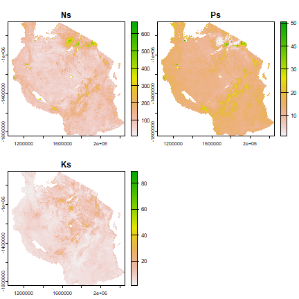
names(supply) <- c("Ns", "Ps", "Ks")
supply
## class : SpatRaster
## dimensions : 1191, 1210, 3 (nrow, ncol, nlyr)
## resolution : 1000, 1000 (x, y)
## extent : 1037375, 2247375, -1841875, -650875 (xmin, xmax, ymin, ymax)
## coord. ref. : +proj=laea +lat_0=5 +lon_0=20 +x_0=0 +y_0=0 +datum=WGS84 +units=m +no_defs
## source(s) : memory
## names : Ns, Ps, Ks
## min values : 8.283516, 1.0000, 1.00
## max values : 742.129666, 52.7725, 89.25
plot(supply)
Water limited yield
For attainable yield, we use a raster of water-limited yield estimated by the GYGA project.
Ya <- reagro_data("TZA_YW")
Running QUEFTS
library(Rquefts)
maize <- quefts_crop("Maize")
fertilizer <- list(N=64, P=20, K=0)
q <- quefts(crop=maize, fert=fertilizer)
In this example, 64 kg/ha of N and 20 kg/ha of P comes from using 100 kg/ha of Urea and 100 kg/ha of DAP.
yield <- rast(Ya)
values(yield) <- run(q, supply, Ya)
## Warning: [setValues] values were recycled
plot(yield)