QUEFTS
Introduction
This chapter describes the QUEFTS model. QUEFTS stands for
QUantitative Evaluation of the Fertility of Tropical Soils. It is a
simple rule-based model to estimate crop yield given a few soil
properties and the amount of fertilizer applied, or to estimate the
amount of fertilizer needed to reach a particular yield.
QUEFTS was first described in: B.H. Janssen, F.C.T. Guiking, D. van der Eijk, E.M.A. Smaling, J. Wolf and H.van Reuler. 1990. A system for quantitative evaluation of the fertility of tropical soils (QUEFTS).Geoderma 46: 299-318.
To run the model, you need soil and crop parameters, as well as the amount of fertilizer applied, and the attainable crop production. In this context, the attainable production that is either the maximum production in the absence of nutrient limitation.
Technical background
Potential supply of nutrients
QUEFTS uses soil properties to estimate the potential soil supply of the three macro-nutrients nitrogen (N), phosphorus (P) and potassium (K). Other nutrients are ignored here, although the model could be extended to include them.
Potential soil supply is estimated based on relationships between chemical topsoil properties and the maximum quantity of those nutrients that can be taken up by the crop, if no other nutrients are limiting growth.
The potential soil supply is crop and soil specific and can be determined through experiments with different levels of the target nutrients and all other nutrients are in ample supply. The target nutrient thus becomes the most limiting, and the maximum soil supply of that nutrient can be estimated from the crop’s nutrient uptake, and related to soil properties such as pH, and organic carbon content (Janssen et al., 1990).
The equations used by QUEFTS to calculate the potential supply of nutrients from soil properties were derived from empirical data of field trials in Suriname and Kenya. They are thought to be applicable to well drained, deep soils, that have a pH(H20) in the range 4.5-7.0, and values for organic carbon below 70 g/kg, P-Olsen below 30 mg/kg and exchangeable potassium below 30 mmol/kg.
Let’s have a look at this relationship. Below we compute the nutrient supply for a range of pH values, and given different levels for the other soil properties. The other soil properties are organic C (SOC=10 g/kg), exchangabke potassium (Kex=1), and Phosphorus extracted with the Olsen method (Polsen = 1 mg/kg) .
We compute nutrient supply across these pH ranges, given fixed values fir
library(Rquefts)
# range of pH values
ph <- seq(4, 8, 1)
s <- nutSupply(ph, SOC=15, Kex=1, Polsen=1)
cbind(ph, s)
##      ph N_base_supply P_base_supply K_base_supply
## [1,]  4          25.5         0.000     29.032258
## [2,]  5          51.0         3.125     22.580645
## [3,]  6          76.5         5.750     16.129032
## [4,]  7         102.0         3.125      9.677419
## [5,]  8         127.5         0.000      3.225806
We now the same thing, but with smaller steps if of pH values, to make smooth plots, and with different levels of the other properties.
ph <- seq(4, 8, 0.25)
# three combinations
s1 <- nutSupply(ph, SOC=15, Kex=5, Polsen=5)
s2 <- nutSupply(ph, SOC=30, Kex=10, Polsen=10)
s3 <- nutSupply(ph, SOC=45, Kex=20, Polsen=20)
We can use the results to make plots of the effect of pH on N, P and K supply, for these three situations (low, medium and high levels of organic matter, exchangeble K, and Olsen-P).
par(mfrow=c(1,3))

for (supply in c("N_base_supply", "P_base_supply", "K_base_supply")) {
  plot(ph, s3[,supply], xlab="pH", ylab=paste(supply, "(kg/ha)"), type="l", ylim=c(0,max(s3[,supply])))
  lines(ph, s2[,supply])
  lines(ph, s1[,supply])
}
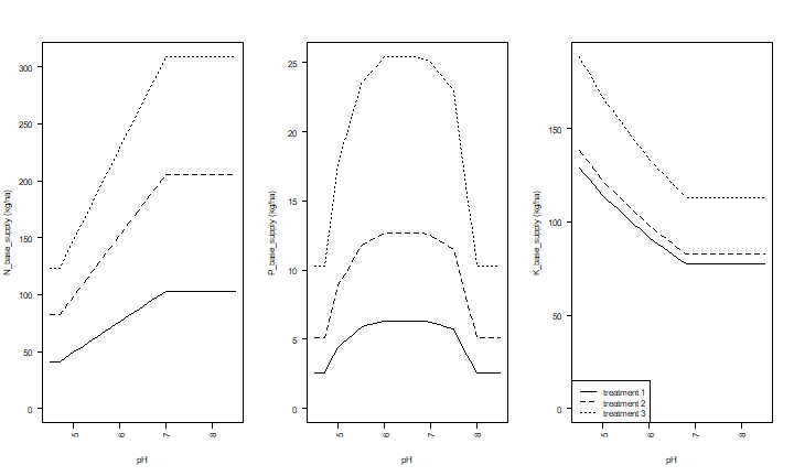
This shows that P-supply is highest at a pH=6, for any Olsen-P level – reflecting the fact that phosphoros becomes less available to plants at low or high pH. N-supply decreases with pH (given the amount of soil Carbon), and K-supply increases with pH (given the amount of exchangeble K).
Now let’s look at the nutrient supply for varying levels of Soil Carbon.
# unit is g/kg
om <- seq(0, 70, 5)
# three combinations
s1 <- nutSupply(pH=5.5, SOC=om, Kex=5, Polsen=5)
s2 <- nutSupply(pH=5.5, SOC=om, Kex=10, Polsen=10)
s3 <- nutSupply(pH=5.5, SOC=om, Kex=20, Polsen=20)

# and plot
par(mfrow=c(1,3))
for (supply in c("N_base_supply", "P_base_supply", "K_base_supply")) {
  plot(om, s3[,supply], xlab="Soil Carbon (g/kg)", ylab=paste(supply, "(kg/ha)"), type="l", ylim=c(0,max(s3[,supply])))
  lines(om, s2[,supply])
  lines(om, s1[,supply])
}
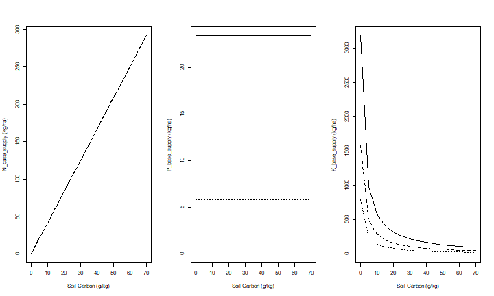
This shows that organic carbon has a strong positive effect on available N and P, but a negative effect on K availability (given the amount of exchangable K).
We can assume that these relationships are robust, at least for the conditions that they were designed for (pH(H20) 4.5-7.0, organic carbon below 70 g/kg, P-Olsen below 30 mg/kg and exchangeable potassium below 30 mmol/kg). But with experimental data, these relationships could be re-estimated, also for other conditions.
Actual nutrient uptake
The actual uptake of each nutrient is estimated as a function of the potential soil supply of that nutrient, taking into account the potential soil supply of the other two nutrients, and the maximum nutrient concentrations in the vegetative and generative organs of the crop.
The estimated uptake of nitrogen, phosphorus, and potassium is used to estimated biomass production ranges for each nutrient. For each pair of nutrients two yield estimates are calculated. For example the yield for the actual N uptake is computed dependent on the yield range for the P and the for the K uptake. This leads to six combinations describing the uptake of one nutrient given maximum dilution or accumulation of another.
The nutrient-limited yield is then estimated by averaging the six yield estimates for paired nutrients. An estimate based on two nutrients may not exceed the upper limit of the yield range of the third nutrient, that is, the concentration of a nutrient can not be lower than its maximum dilution level. Neither may the yield estimates exceed the spacified maximum (attainable) production.
Create and run a model
The first step is to create a model. You can create a model with default parameters like this
library(Rquefts)
q <- quefts()
And then run the model
run(q)
##   leaf_lim   stem_lim  store_lim   N_supply   P_supply   K_supply   N_uptake
## 1928.19667 1928.19667 3756.94929   90.00000   11.00000   90.00000   81.66872
##   P_uptake   K_uptake      N_gap      P_gap      K_gap
##   10.88951   77.38765   60.00000  205.00000    0.00000
You can also initialize a model with parameters of you choice. Here we use the default parameters for barley, and we set the attainable biomass accuumlation at 2200 kg/ha for leaves, 2700 kg/ha for stems, and 4800 kg/ha for grain. We set the seasonlength to 110 days.
soiltype <- quefts_soil()
barley <- quefts_crop('Barley')
fertilizer <- list(N=50, P=0, K=0)
biomass <- list(leaf_att=2200, stem_att=2700, store_att=4800, SeasonLength=110)
q <- quefts(soiltype, barley, fertilizer, biomass)
If the crop has biological nitrogen fixation (in symbiosis with Rhizobium) you can use the NFIX parameter to determine the fraction of the total nitrogen supply that is supplied by biological fixation. Note that NFIX is a constant, while in reality nitrogen fixation is amongst other things dependent on the amount of mineral nitrogen available in the soil.
Explore
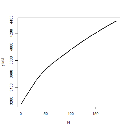
Let’s have a look how rice yield is affected by N fertilization. First set up some parameters
rice <- quefts_crop("Rice")
q <- quefts(crop=rice)
q$leaf_att <- 2651
q$stem_att <- 5053
q$store_att <- 8208
fert(q) <- list(N=0, P=0, K=0)
N <- seq(1, 200, 10)
Now set up an output matrix, and run the model for each fertlizer application.
results <- matrix(nrow=length(N), ncol=12)
colnames(results) <- names(run(q))
for (i in 1:length(N)) {
    q["N"] <- N[i]
    results[i,] <- run(q)
}
yield <- results[,"store_lim"]
yield
##  [1] 3162.406 3286.369 3402.153 3509.081 3604.427 3678.601 3744.550 3802.401
##  [9] 3858.675 3913.410 3966.648 4018.424 4068.778 4117.746 4165.363 4211.664
## [17] 4256.683 4300.454 4343.009 4384.379
And make a plot
plot(N, yield, type="l", lwd=2)
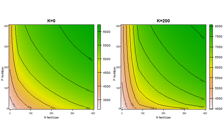
We can also look at interactions by changing two nutrients. Here we change N and P fertilization levels, while keeping K constant (either 0 or 200 mmol/kg)
f <- expand.grid(N=seq(0,400,10), P=seq(0,400,10), K=c(0,200))
x <- rep(NA, nrow(f))
for (i in 1:nrow(f)) {0
    q$N <- f$N[i]
    q$P <- f$P[i]
    q$K <- f$K[i]
    x[i] <- run(q)["store_lim"]
}
x <- cbind(f, x)
head(x)
##    N P K        x
## 1  0 0 0 3149.509
## 2 10 0 0 3274.362
## 3 20 0 0 3390.910
## 4 30 0 0 3498.943
## 5 40 0 0 3596.358
## 6 50 0 0 3671.320
To display the results we can treat the values as a raster
library(raster)
r0 <- rasterFromXYZ(x[x$K==0, -3])
r200 <- rasterFromXYZ(x[x$K==200, -3])

par(mfrow=c(1,2))
plot(r0, xlab="N fertilizer", ylab="P fertilizer", las=1, main="K=0")
contour(r0, add=TRUE)
plot(r200, xlab="N fertilizer", ylab="P fertilizer", las=1, main="K=200")
contour(r200, add=TRUE)
Callibration
If you have your own experimental data, you could callibrate QUEFTS. Here I illustrate some basic approaches that can be used for callibration.First I generate some data.
set.seed(99)
yldfun <- function(N, noise=TRUE) { 1000 +  500* log(N+1)/3 + noise * runif(length(N), -500, 500) }
N <- seq(0,300,25)
Y <- replicate(10, yldfun(N))
obs <- cbind(N, Y)
We will use Root Mean Square Error (RMSE) to assess model fit.
RMSE <- function(obs, pred) sqrt(mean((obs - pred)^2))
Let’s see how good the default parameters work for us.
q <- quefts()
q$P <- 0
q$K <- 0

results <- matrix(nrow=length(N), ncol=12)
colnames(results) <- names(run(q))
for (i in 1:length(N)) {
    q$N <- N[i]
    results[i,] <- run(q)
}

yield <- results[,'store_lim']
RMSE(obs[,-1], yield)
## [1] 1868.019
The RMSE is quite high.
We create a function to minimize with the optimizer. Here I try to improve the model by altering four parameters.
vars <- c('soil$N_base_supply', 'soil$N_recovery', 'crop$NminStore', 'crop$NmaxStore')
f <- function(p) {
    if (any (p < 0)) return(Inf)
    if (p['crop$NminStore'] >= p['crop$NmaxStore']) return(Inf)
    if (p['soil$N_recovery'] > .6 | p['soil$N_recovery'] < .3) return(Inf)
    q[names(p)] <- p
    pred <- run(q)
    RMSE(obs[,-1], pred['store_lim'])
}

# try the function with some initial values
x <- c(50, 0.5,  0.011, 0.035)
names(x) <- vars
f(x)
## [1] 1573.818
Now tht we have a working functon, we can use optimization methods to try to find the combination of parameter values that is the best fit to our data.
par <- optim(x, f)
# RMSE
par$value
## [1] 1478.384
# optimal parameters
par$par
## soil$N_base_supply    soil$N_recovery     crop$NminStore     crop$NmaxStore
##         0.01398939         0.59768399        26.37808069        37.05140516