Crop-cut data: India
In this chapter we pre-process rice crop-cut data from Odisha, collected by Iftikar et al., 2017:
Wasim Iftikar; Nabakishore Parida; Vivek Kumar; Narayan Chandra Banik; Amit Mishra, 2017, “Odisha Rice Crop Cut Data 2013 - 2016”, hdl:11529/11111, CIMMYT Research Data & Software Repository Network, V2
The data are avaialble on the CIMMYT data repository https://data.cimmyt.org/dataset.xhtml?persistentId=hdl:11529/11111
We are not reproducing a paper here, we are just finding out how to pre-process the data so that they can be used for further analysis.
Get the data
We use the agro package to download the data.
ff <- agro::get_data_from_uri("hdl:11529/11111", ".")
ff
## [1] "./hdl_11529_11111/CSISA_OD_RiceCropCut_AllYearRawDataFinal.csv"
## [2] "./hdl_11529_11111/CSISA_OD_RiceCropCut_MetaSheet_1.csv"
We have two .csv files. One with data, and one with metadata.
ff[1]
## [1] "./hdl_11529_11111/CSISA_OD_RiceCropCut_AllYearRawDataFinal.csv"
d <- read.csv(ff[1], stringsAsFactors = FALSE)
dim(d)
## [1] 816  33
There are 816 records and 33 variables, with these names
colnames(d)
##  [1] "Year"                "Season"              "District_Name"
##  [4] "FID"                 "Latitude"            "Longitude"
##  [7] "CEM"                 "VAR"                 "DOS"
## [10] "DOT"                 "Seed_Rate"           "DAP_Total"
## [13] "MoP_Total"           "Urea_Total"          "Urea_1_Top"
## [16] "MoP_1_Top"           "Urea_2_Top"          "MoP_2_Top"
## [19] "Urea_3_Top"          "MoP_3_Top"           "Pre_Herbicide_Name"
## [22] "Pre_Herbicide_Amt"   "Post_Herbicide_Name" "Post_Herbicide_Amt"
## [25] "H_Weed_No."          "DOH"                 "TAGB_A"
## [28] "TAGB_B"              "TAGB_C"              "Yield_A"
## [31] "Yield_B"             "Yield_C"             "Gr_Moisture"
At this point it is good to explore the data a bit using functions such
as summary, View, plot and table. For example
table(d$Year)
##
## 2013 2014 2015 2016
##  149  250  201  216
Showing that we have data for four years.
Compute mean yield
We are dealing with crop cut data, and our first interest is in the observed yield. There are three columns with “Yield” in the name. So let’s check these out.
yield <- d[, c("Yield_A", "Yield_B", "Yield_C")]
head(yield)
##   Yield_A Yield_B Yield_C
## 1    2800    2800    2700
## 2    2200    2100    2100
## 3    2100    2000    2040
## 4    2400    2400    2100
## 5    1900    1900    2100
## 6    1500    1420    1400
Look’s good, let’s get the mean yield
y_avg <- rowMeans(yield)
## Error in rowMeans(yield): 'x' must be numeric
Apparently, our yield data are not numeric. Let’s check that.
sapply(yield, class)
##     Yield_A     Yield_B     Yield_C
##   "numeric" "character" "character"
We can change the character fields to numeric
y <- apply(yield, 2, as.numeric)
## Warning in apply(yield, 2, as.numeric): NAs introduced by coercion
## Warning in apply(yield, 2, as.numeric): NAs introduced by coercion
But now we get a warning saying that some values cannot be converted to numbers. Never just ignore warnings like this. You have to investigate why they occur before you can continue. Often this means that there is an error in the data.
Let’s find some of the records that could not be converted.
na_rows <- apply(is.na(y), 1, any)
table(na_rows)
## na_rows
## FALSE  TRUE
##   667   149
nas <- which(na_rows)
head(nas)
## [1] 668 669 670 671 672 673
yield[nas[1:5], ]
##     Yield_A Yield_B Yield_C
## 668   12.50       -       -
## 669   18.00       -       -
## 670   12.00       -       -
## 671   14.08       -       -
## 672   13.00       -       -
Ah, some records only have missing data indicated by "-". Let’s see
if that is connected to the year of data collection.
table(d$Year, na_rows)
##       na_rows
##        FALSE TRUE
##   2013     0  149
##   2014   250    0
##   2015   201    0
##   2016   216    0
It is indeed connected to the year. All records for 2013 have only one yield measurement, all other years have three samples per field.
Instead of continuing, we should see what we can do to allow converting
these data without getting a warning. We should be able to do that by
first replacing the "-" with NA.
yield[yield == "-"] <- NA
y <- apply(yield, 2, as.numeric)
All right, with that problem solved, let’s try again to compute the the
mean yield for each row. Note that we have to use na.rm=TRUE to
avoid getting missing values for 2013.
y_avg <- rowMeans(y, na.rm=TRUE)
To keep all records together, we can add y_avg back to our original
data, data.frame d
d$yield <- y_avg
Let’s see what the yields look like in Odisha:
plot(sort(d$yield))
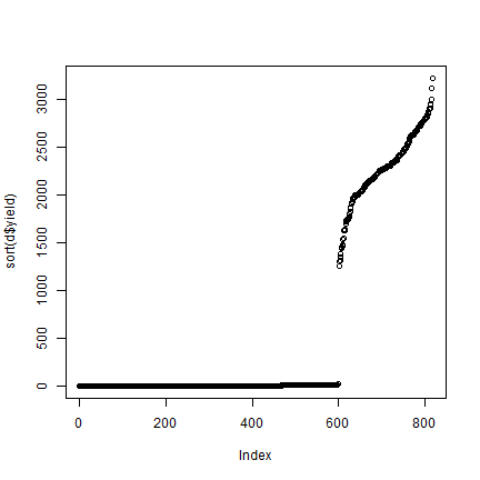
Yikes, that does not look right. Let’s look at the mean yield per year
tapply(d$yield, d$Year, mean, na.rm=TRUE)
##         2013         2014         2015         2016
##    9.5491275    2.6973987    0.5751542 2283.5231481
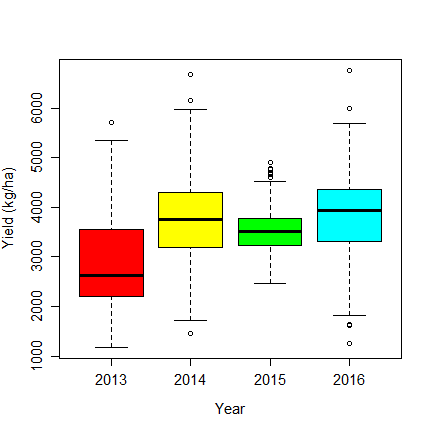
Or as a boxplot
boxplot(yield~Year, data=d)
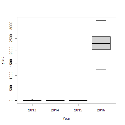
These are wildly different numbers. Perhaps different units? Let’s consult the metadata!
Metadata
The second file contains metadata (at least that is what the file name suggests).
ff[2]
## [1] "./hdl_11529_11111/CSISA_OD_RiceCropCut_MetaSheet_1.csv"
md <- read.csv(ff[2], stringsAsFactors = FALSE, header=FALSE)
head(md)
##             V1                                               V2
## 1      Project Cereal Systems Initiative for South Asia (CSISA)
## 2        Donor                                     BMGF & USAID
## 3      Country                                            India
## 4          Hub                                           Odisha
## 5 DocumentName                                      RiceCropCut
## 6 ProducedYear                                             2017
This .csv file did not have a “header” (no column/variable names),
so we add them for clarity
colnames(md) <- c("var", "value")
Let’s look for the discription of our yield variables
i <- grep("Yield", md$var)
i
## [1] 48 49 50
md$var[i]
## [1] "Yield_A " "Yield_B"  "Yield_C"
Note the space trailing “Yield_A”? Additional whitespace (space, tab) like that can be difficult to spot and cause a lot trouble later on, so let’s remove all leading or trailing whitespace first. This is really very important for data processing, not so much for the meta-data, but it does not hurt to be careful.
md <- apply(md, 2, trimws)
# apply returns a matrix, let's keep a data.frame (always with stringsAsFactors=FALSE)
md <- data.frame(md, stringsAsFactors = FALSE)
Now inspect the values
md$value[i]
## [1] "Grain weight at spot A\nYear 2013 - 5X5 sq meter in Kg\nYear 2014 - 2X2.5 sq meter in Kg\nYear 2015 - 1X1 sq meter in gm\nYear 2016 - 2X2 sq meter in gm"
## [2] "Grain weight at spot B\nYear 2013 - 5X5 sq meter in Kg\nYear 2014 - 2X2.5 sq meter in Kg\nYear 2015 - 1X1 sq meter in gm\nYear 2016 - 2X2 sq meter in gm"
## [3] "Grain weight at spot C\nYear 2013 - 5X5 sq meter in Kg\nYear 2014 - 2X2.5 sq meter in Kg\nYear 2015 - 1X1 sq meter in gm\nYear 2016 - 2X2 sq meter in gm"
The variables are the same, except for the “spot A”, “spot B”, and “spot
C” bits. You can check that by removing the first part of each value and
then taking the unique value. Note that in the pattern provided to the
gsub function below the . serves a “wild card”: it matches any
character. Also note the presence of \n which represents a line
break.
ymd <- gsub("Grain weight at spot .\n", "", md$value[i])
ymd <- unique(ymd)
ymd
## [1] "Year 2013 - 5X5 sq meter in Kg\nYear 2014 - 2X2.5 sq meter in Kg\nYear 2015 - 1X1 sq meter in gm\nYear 2016 - 2X2 sq meter in gm"
To show the effect of the line breaks, and to allow for easier reading,
we can use cat
cat(ymd)
## Year 2013 - 5X5 sq meter in Kg
## Year 2014 - 2X2.5 sq meter in Kg
## Year 2015 - 1X1 sq meter in gm
## Year 2016 - 2X2 sq meter in gm
All right, so different years have different units. That is unexpected. In most cases all values of a variable (column) in a data set have the same unit. But, unfortunately, that is not always the case — and that can lead to a lot of errors (e.g. temperature in °F and °C, or elevation in meter and feet). Sometimes the unit is stored in another column, but in this case it is not, so we shall do that ourselves. Here we need to adjust for both the area harvested and the unit of mass used.
First make a table of the unit by year. In this case I would do that “by hand”:
units <- data.frame(Year=2013:2016, area=c(25, 2*2.5 ,1 , 4), tokg=c(1,1,1000,1000))
units
##   Year area tokg
## 1 2013   25    1
## 2 2014    5    1
## 3 2015    1 1000
## 4 2016    4 1000
The tokg variable indicates by how much the number needs to be
divided to get kg (from g).
We already saw that in 2013 there was only one sample per field, but now we see that the plots were larger. So it appears that there was a change in the protocol from one larger sample to three smaller samples.
Compute yield per ha
We are now ready to adjust the yield data from the raw values to a
single unit (we’ll use kg/ha). First we merge the data d with the
new table units. When using merge you have to be careful that
you do not loose records because of bad matching of values. So I check
the number of records before and after merging.
dim(d)
## [1] 816  34
dm <- merge(d, units, by="Year")
dim(dm)
## [1] 816  36
The resulting data
head(dm[, c("Year", "yield", "area", "tokg")])
##   Year yield area tokg
## 1 2013 12.50   25    1
## 2 2013 18.00   25    1
## 3 2013 12.00   25    1
## 4 2013 14.08   25    1
## 5 2013 13.00   25    1
## 6 2013 11.50   25    1
tail(dm[, c("Year", "yield", "area", "tokg")])
##     Year    yield area tokg
## 811 2016 2278.333    4 1000
## 812 2016 2449.333    4 1000
## 813 2016 2473.333    4 1000
## 814 2016 2338.667    4 1000
## 815 2016 2245.333    4 1000
## 816 2016 2434.000    4 1000
table(dm[, c("Year", "area")])
##       area
## Year     1   4   5  25
##   2013   0   0   0 149
##   2014   0   0 250   0
##   2015 201   0   0   0
##   2016   0 216   0   0
Compute yield in kg/ha
dm$yha <- (10000 / dm$area) * (dm$yield / dm$tokg)
Let’s again check the numbers
tapply(dm$yha, dm$Year, mean, na.rm=TRUE)
##        2013        2014        2015        2016
## 3819.651007 5394.797333    5.751542 5708.807870
The yield for 2015 is much too low now whereas the other values are plausible rice yields in kg/ha. So I assume that the 2015 data were, in fact, in kg/ha, and not in g/ha.
dm$tokg[dm$Year==2015] <- 1
dm$yha <- (10000 / dm$area) * (dm$yield / dm$tokg)
Now the yield data look plausible
tapply(dm$yha, dm$Year, mean, na.rm=TRUE)
##     2013     2014     2015     2016
## 3819.651 5394.797 5751.542 5708.808
A final step is to correct for variation in moisture content. We can use
the field Gr_Moisture but there are again missing values.
dm$Gr_Moisture[dm$Gr_Moisture == "-"] <- NA
dm$Gr_Moisture <- as.numeric(dm$Gr_Moisture)
table(dm$Year, is.na(dm$Gr_Moisture))
##
##        FALSE TRUE
##   2013   149    0
##   2014   156   94
##   2015   200    1
##   2016   216    0
boxplot(Gr_Moisture~Year, data=dm, col=rainbow(6), ylab="Yield (kg/ha)", cex.axis=1.25, cex.lab=1.25)
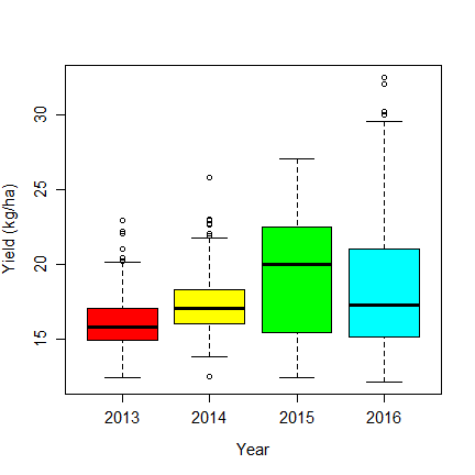
The table shows that there is 1 missing value in 2015, and 94 in 2014. The boxplot shows different moisture contents by years, so lets replace the missing values with the mean value for each year. Compute the mean values:
moisture <- aggregate(dm[, "Gr_Moisture", drop=FALSE], dm[, "Year", drop=FALSE], mean, na.rm=TRUE)
colnames(moisture)[2] <- "avg_moisture"
moisture
##   Year avg_moisture
## 1 2013     16.15705
## 2 2014     17.34359
## 3 2015     19.43600
## 4 2016     18.56995
Merge with the data
dim(dm)
## [1] 816  37
dm <- merge(dm, moisture, by="Year")
dim(dm)
## [1] 816  38
Find and replace the missing values
i <- is.na(dm$Gr_Moisture)
dm$Gr_Moisture[i] <- dm$avg_moisture[i]
table(is.na(dm$Gr_Moisture))
##
## FALSE
##   816
boxplot(Gr_Moisture~Year, data=dm, col=rainbow(6), ylab="Yield (kg/ha)", cex.axis=1.25, cex.lab=1.25)
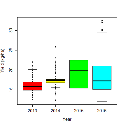
The boxplot shows that the distribution has changed for 2014 — as there are now 97 values with the same (mean) value.
For rice, standard moisture content is 12%. We can compute it like this
dm$yha <- 12 * dm$yha / dm$Gr_Moisture
boxplot(yha~Year, data=dm, col=rainbow(6), ylab="Yield (kg/ha)", cex.axis=1.25, cex.lab=1.25)
Fertilizer
These are the fertilizer variables
fert <- c("DAP_Total", "MoP_Total", "Urea_Total", "Urea_1_Top", "MoP_1_Top", "Urea_2_Top", "MoP_2_Top", "Urea_3_Top", "MoP_3_Top")
md[md$var %in% fert, ]
##           var
## 30  DAP_Total
## 31  MoP_Total
## 32 Urea_Total
## 33 Urea_1_Top
## 34  MoP_1_Top
## 35 Urea_2_Top
## 36  MoP_2_Top
## 37 Urea_3_Top
## 38  MoP_3_Top
##                                                                                  value
## 30 Total amount of Di-ammonium Phosphate used in Kg per acre throughout the crop cycle
## 31      Total amount of Murate of Potash used in Kg per acre throughout the crop cycle
## 32                  Total amount of Urea used in Kg per acre throughout the crop cycle
## 33                Amount of Urea used in Kg per acre at the time of first top dressing
## 34    Amount of Murate of Potash used in Kg per acre at the time of first top dressing
## 35               Amount of Urea used in Kg per acre at the time of second top dressing
## 36   Amount of Murate of Potash used in Kg per acre at the time of second top dressing
## 37                Amount of Urea used in Kg per acre at the time of third top dressing
## 38    Amount of Murate of Potash used in Kg per acre at the time of third top dressing
A check to see if there are values. Get the max value for each variable by year.
aggregate(dm[, fert], dm[,"Year",drop=FALSE], max, na.rm=TRUE)
## Warning in FUN(X[[i]], ...): no non-missing arguments to max; returning -Inf
## Warning in FUN(X[[i]], ...): no non-missing arguments to max; returning -Inf
## Warning in FUN(X[[i]], ...): no non-missing arguments to max; returning -Inf
## Warning in FUN(X[[i]], ...): no non-missing arguments to max; returning -Inf
## Warning in FUN(X[[i]], ...): no non-missing arguments to max; returning -Inf
## Warning in FUN(X[[i]], ...): no non-missing arguments to max; returning -Inf
## Warning in FUN(X[[i]], ...): no non-missing arguments to max; returning -Inf
## Warning in FUN(X[[i]], ...): no non-missing arguments to max; returning -Inf
## Warning in FUN(X[[i]], ...): no non-missing arguments to max; returning -Inf
##   Year DAP_Total MoP_Total Urea_Total Urea_1_Top MoP_1_Top Urea_2_Top MoP_2_Top
## 1 2013        75      50.0          0         60         0         25         0
## 2 2014       100       0.0          0         40        25         50        30
## 3 2015       100      62.5         65          0         0          0         0
## 4 2016      -Inf      -Inf       -Inf       -Inf      -Inf       -Inf      -Inf
##   Urea_3_Top MoP_3_Top
## 1         40         0
## 2         50        30
## 3          0         0
## 4       -Inf      -Inf
Lots of warnings because there are no fertilizer data for 2016. Thus all
values for that year are NA and you cannot get a max value in
that case for a group that only has NA. You could use this function
function(i) ifelse(all(is.na(i)), NA, max(i, na.rm=TRUE))) instead,
to get rid of the warnings, but at the cost of tremendous verbosity.
All right, 2016 is out. Alose notice that in 2013 and 2014 the maximum
value of Urea_Total is 0, whereas there Urea_Top variables show that
this should not be the case. The opposite is the case for 2015: there is
Urea_Total data, but no data for the split applications.
The situation is similar for MoP_Total, with no values in 2014.
Let’s fix that.
i <- dm$Year %in% c(2013, 2014)
sum(i)
## [1] 399
dm$Urea_Total[i] <- rowSums(dm[i, c("Urea_1_Top", "Urea_2_Top", "Urea_3_Top")])
j <- dm$Year == 2014
sum(j)
## [1] 250
dm$MoP_Total[j] <- rowSums(dm[j, c("MoP_1_Top", "MoP_2_Top", "MoP_3_Top")])
Let’s check
df <- dm[dm$Year != 2016, ]
aggregate(df[, fert[1:3]], df[,"Year",drop=FALSE], mean, na.rm=TRUE)
##   Year DAP_Total MoP_Total Urea_Total
## 1 2013  32.59732  26.63793   36.83893
## 2 2014  25.76400  15.54800   32.51600
## 3 2015  36.30597  27.38065   35.73134