Crop mapping with satellite data
Benson Kenduiywo
Background
Mapping the distribution of crops is important for several applications. A problem with using remote sensing data for crop mapping is the presence of clouds. As crops are typically grown in the rainy seasons, they may be difficult to detect with the commonly used optical reflectance data. Radar remote sensing data is not affected by weather conditions (or the presence of daylight), and that makes it a very interesting alternative to optical data. Here we use Sentinel-1 radar data to map different crop types in Kitale, Kenya. We build on the approaches introduced in the introduction to remote sensing tutorial, but we focus on other aspecs (feature creation and model evaluation).
TO DO: add link to page on general Sentinel info (some technical specs and where to get)
Data
We provide a set of processed Sentinel-1 VV and VH polarized images. To learn about the basics of radar visit EO College, SERVIR SAR HANDBOOK or European Space Agency (ESA) tutorials. The images are ground range products with equidistant pixel spacing. They were radiometrically calibrated to \(\sigma_0\). All images were co-registered and transformed to the UTM-36N and WGS1984 datum coordinate reference system.
Here is how you can get the Sentinel data for this tutorial.
workdir <- file.path(dirname(tempdir()))
datadir <- file.path(workdir, "agrin/sentinel")
dir.create(datadir, showWarnings = FALSE, recursive=TRUE)
library(agrin)
datadir
## [1] "c:/temp/agrin/sentinel"
ff <- crop_data("sentinel1", datadir)
head(ff)
## [1] "c:/temp/agrin/sentinel/S1A_IW_A_GRDH_VH_2015_09_15_Clip.tif"
## [2] "c:/temp/agrin/sentinel/S1A_IW_A_GRDH_VH_2015_12_20_Clip.tif"
## [3] "c:/temp/agrin/sentinel/S1A_IW_A_GRDH_VV_2015_03_07_Clip.tif"
## [4] "c:/temp/agrin/sentinel/S1A_IW_A_GRDH_VV_2015_03_31_Clip.tif"
## [5] "c:/temp/agrin/sentinel/S1A_IW_A_GRDH_VV_2015_05_18_Clip.tif"
## [6] "c:/temp/agrin/sentinel/S1A_IW_A_GRDH_VV_2015_06_11_Clip.tif"
Here is just a trick to skip some preprocessing if that has already been done
imgfile <- file.path(workdir, "img.tif")
imgexists <- file.exists(imgfile)
You can use the grep funtion to get the VV polarized images.
fvv <- grep("VV", ff, value = TRUE)
i <- order(substr(basename(fvv), 15, 27))
fvv <- fvv[i]
fvv
##  [1] "c:/temp/agrin/sentinel/S1A_IW_A_GRDH_VV_2015_03_07_Clip.tif"
##  [2] "c:/temp/agrin/sentinel/S1A_IW_D_GRDH_VV_2015_03_14_Clip.tif"
##  [3] "c:/temp/agrin/sentinel/S1A_IW_D_GRDH_VV_2015_03_21_Clip.tif"
##  [4] "c:/temp/agrin/sentinel/S1A_IW_A_GRDH_VV_2015_03_31_Clip.tif"
##  [5] "c:/temp/agrin/sentinel/S1A_IW_D_GRDH_VV_2015_04_07_Clip.tif"
##  [6] "c:/temp/agrin/sentinel/S1A_IW_D_GRDH_VV_2015_04_14_Clip.tif"
##  [7] "c:/temp/agrin/sentinel/S1A_IW_D_GRDH_VV_2015_05_01_Clip.tif"
##  [8] "c:/temp/agrin/sentinel/S1A_IW_A_GRDH_VV_2015_05_18_Clip.tif"
##  [9] "c:/temp/agrin/sentinel/S1A_IW_D_GRDH_VV_2015_06_01_Clip.tif"
## [10] "c:/temp/agrin/sentinel/S1A_IW_A_GRDH_VV_2015_06_11_Clip.tif"
## [11] "c:/temp/agrin/sentinel/S1A_IW_D_GRDH_VV_2015_06_25_Clip.tif"
## [12] "c:/temp/agrin/sentinel/S1A_IW_A_GRDH_VV_2015_07_05_Clip.tif"
## [13] "c:/temp/agrin/sentinel/S1A_IW_D_GRDH_VV_2015_07_12_Clip.tif"
## [14] "c:/temp/agrin/sentinel/S1A_IW_D_GRDH_VV_2015_07_19_Clip.tif"
## [15] "c:/temp/agrin/sentinel/S1A_IW_A_GRDH_VV_2015_07_29_Clip.tif"
## [16] "c:/temp/agrin/sentinel/S1A_IW_A_GRDH_VV_2015_08_22_Clip.tif"
## [17] "c:/temp/agrin/sentinel/S1A_IW_D_GRDH_VV_2015_08_29_Clip.tif"
## [18] "c:/temp/agrin/sentinel/S1A_IW_A_GRDH_VV_2015_09_15_Clip.tif"
## [19] "c:/temp/agrin/sentinel/S1A_IW_A_GRDH_VV_2015_10_09_Clip.tif"
## [20] "c:/temp/agrin/sentinel/S1A_IW_D_GRDH_VV_2015_10_16_Clip.tif"
## [21] "c:/temp/agrin/sentinel/S1A_IW_A_GRDH_VV_2015_11_02_Clip.tif"
## [22] "c:/temp/agrin/sentinel/S1A_IW_D_GRDH_VV_2015_11_09_Clip.tif"
## [23] "c:/temp/agrin/sentinel/S1A_IW_D_GRDH_VV_2015_11_16_Clip.tif"
## [24] "c:/temp/agrin/sentinel/S1A_IW_A_GRDH_VV_2015_11_26_Clip.tif"
## [25] "c:/temp/agrin/sentinel/S1A_IW_D_GRDH_VV_2015_12_10_Clip.tif"
## [26] "c:/temp/agrin/sentinel/S1A_IW_A_GRDH_VV_2015_12_20_Clip.tif"
vv <- rast(fvv)
# make prettier (shorter) layer names
names(vv) <- substr(names(vv), 15, 27)
names(vv)
##  [1] "VV_2015_03_07" "VV_2015_03_14" "VV_2015_03_21" "VV_2015_03_31"
##  [5] "VV_2015_04_07" "VV_2015_04_14" "VV_2015_05_01" "VV_2015_05_18"
##  [9] "VV_2015_06_01" "VV_2015_06_11" "VV_2015_06_25" "VV_2015_07_05"
## [13] "VV_2015_07_12" "VV_2015_07_19" "VV_2015_07_29" "VV_2015_08_22"
## [17] "VV_2015_08_29" "VV_2015_09_15" "VV_2015_10_09" "VV_2015_10_16"
## [21] "VV_2015_11_02" "VV_2015_11_09" "VV_2015_11_16" "VV_2015_11_26"
## [25] "VV_2015_12_10" "VV_2015_12_20"
vv
## class       : SpatRaster
## dimensions  : 982, 783, 26  (nrow, ncol, nlyr)
## resolution  : 10, 10  (x, y)
## extent      : 705883.3, 713713.3, 112681.4, 122501.4  (xmin, xmax, ymin, ymax)
## coord. ref. : +proj=utm +zone=36 +datum=WGS84 +units=m +no_defs
## data sources: c:/temp/agrin/sentinel/S1A_IW_A_GRDH_VV_2015_03_07_Clip.tif
##               c:/temp/agrin/sentinel/S1A_IW_D_GRDH_VV_2015_03_14_Clip.tif
##               c:/temp/agrin/sentinel/S1A_IW_D_GRDH_VV_2015_03_21_Clip.tif
##               c:/temp/agrin/sentinel/S1A_IW_A_GRDH_VV_2015_03_31_Clip.tif
##               c:/temp/agrin/sentinel/S1A_IW_D_GRDH_VV_2015_04_07_Clip.tif
##               c:/temp/agrin/sentinel/S1A_IW_D_GRDH_VV_2015_04_14_Clip.tif
##               ... and 20 more sources
## names       : VV_2015_03_07, VV_2015_03_14, VV_2015_03_21, VV_2015_03_31, VV_2015_04_07, VV_2015_04_14, ...
## min values  :     -23.63815,     -24.24532,     -23.84251,     -24.12050,     -21.34933,     -22.59983, ...
## max values  :     11.090298,     18.059062,      8.262378,     12.798749,     20.114488,      7.086701, ...
Repeat the steps for vh polarization.
fvh <- grep("VH", ff, value = TRUE)
i <- order(substr(basename(fvh), 15, 27))
fvh <- fvh[i]
vh <- rast(fvh)
names(vh) <- substr(names(vh), 15, 27)
names(vh)
## [1] "VH_2015_04_07" "VH_2015_09_15" "VH_2015_12_20"
We also have ground reference data on crop types.
cropref <- crop_data("crop_ref")
head(cropref)
##          x        y class
## 1 711908.3 117516.4 Maize
## 2 710608.3 113696.4 Maize
## 3 712178.3 116916.4 Maize
## 4 711978.3 120526.4 Maize
## 5 710858.3 115086.4 Maize
## 6 711068.3 119616.4 Maize
table(cropref$class)
##
##   Grass   Maize Pasture   Wheat
##     500     500     500     500
Create a SpatVector object
vecref <- vect(cropref[,1:2], att=cropref, crs=crs(vv))
vecref
## class       : SpatVector
## geometry    : points
## elements    : 2000
## extent      : 705928.3, 713278.3, 112916.4, 122286.4  (xmin, xmax, ymin, ymax)
## coord. ref. : +proj=utm +zone=36 +datum=WGS84 +units=m +no_defs
## names       : x, y, class
spplot(vecref, "class")
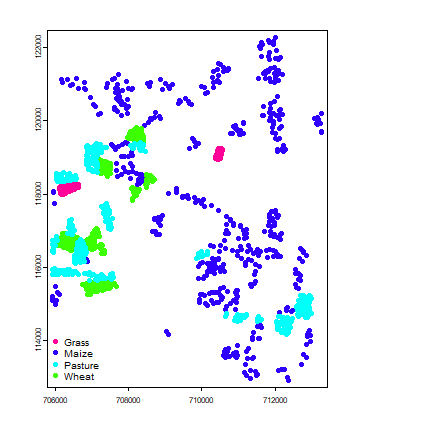
As you can see, the points were generated by sampling within fields.
Feature creation
We have “raw” time series satellite data, and many more images for VV than for VH. We can use these data to build a model to predict crop types, but oftentimes we prefer to compute new “features” (predictor variables) from the raw data. These new features should typically reduce the number of variables (images), while capturing perhaps more of the variation in the data.
Here is function to compute features. It takes a multilayer object x
to create new layers.
compFeatures <- function(x, name){
    # standard deviation
    stdev <- stdev(x)
    # quantiles
    quant <- app(x, function(i) quantile(i, c(.1, .25, .5, .75, .9)))
    # trend
    n <- nlyr(x)
    trend <- 100 * (mean(x[[1:5]] - mean(x[[(n-4):n]])))
    feat <- c(quant, stdev, trend)
    names(feat) <- paste0(name, c(".1", ".25", ".5", ".75", ".9", ".sd", "trend"))
    return(feat)
}
Compute seasonal composite features from VV polarized images
fvv <- file.path(workdir, "vv_ft.tif")
if (!file.exists(fvv)) {
vv_ft <- compFeatures(vv, "vv")
writeRaster(vv_ft, fvv)
} else {
vv_ft <- rast(fvv)
}
vv_ft
## class : SpatRaster
## dimensions : 982, 783, 7 (nrow, ncol, nlyr)
## resolution : 10, 10 (x, y)
## extent : 705883.3, 713713.3, 112681.4, 122501.4 (xmin, xmax, ymin, ymax)
## coord. ref. : +proj=utm +zone=36 +datum=WGS84 +units=m +no_defs
## data source : c:/temp/vv_ft.tif
## names : vv.1, vv.25, vv.5, vv.75, vv.9, vv.sd, ...
## min values : -22.1984978, -21.3848591, -20.1580973, -19.2671399, -18.7003231, 0.7816121, ...
## max values : -4.023386, -2.551054, 2.724735, 12.204748, 19.681878, 13.250704, ...
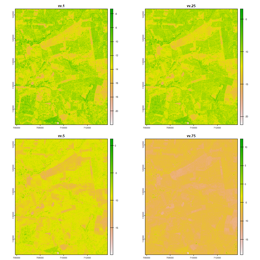
plot(vv_ft)
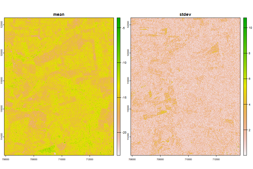
As we only have 4 images for VH polarized images, we cannot use the function above to create features, we’ll just use the mean and the standard deviation.
fvh <- file.path(workdir, "vh_ft.tif")
if (!file.exists(fvh)) {
    sd <- stdev(vh)
    mn <- mean(vh)
    vh_ft <- c(mn, sd)
    names(vh_ft) <- c("mean", "stdev")
    writeRaster(vh_ft, fvh)
} else {
    vh_ft <-- rast(fvh)
}
plot(vh_ft)
 Combine the
 vv and vh features
img <- c(vv_ft, vh_ft)
Model fitting
Various supervised classification algorithms exist, and the choice of algorithm affects the results. Here we used the widely used Random Forests (RF) alogirthm (Breiman 2001).
Random Forests makes predictions using an ensemble of a large number of decision trees. The individual trees are uncorrelated because they are fitted with different subsets of the data. Each tree is fitted with a bootstrapped sample of all the data. A bootstrapped sample is obtained by taking a sample with replacement of the same size as the original data. RandomForest also uses a maximum user-defined number of variables that can randomly selected from to create a node. A different sample is used at each node. Thus each tree has a somewhat different data set and the “best” variable is not always avaiable to create a node. The final prediction (by the forest) is made by averaging the prediction of the individual trees.
The user needs to set the number of trees to build. The more trees, the longer it takes to build the model and to make predictions. Generally, RandomForests models tend to be stable once there are 200 trees (Hastie et al. (2009)).
To train a model, we extract the satellite data for the ground points, using the feature (predictor) data created above.
ref <- extract(img, vecref, drop=TRUE)
ref <- data.frame(class=cropref$class, ref)
head(ref)
##   class      vv.1      vv.25      vv.5     vv.75      vv.9    vv.sd
## 1 Maize -11.05758 -10.481299 -8.789228 -7.538952 -6.349695 1.914231
## 2 Maize -15.24834 -11.633831 -9.693624 -8.460844 -6.773844 3.118843
## 3 Maize -11.99607  -9.939957 -9.011965 -7.437552 -6.433441 2.174761
## 4 Maize -12.43187 -10.576469 -8.890006 -7.028844 -6.291332 2.285031
## 5 Maize -11.04900  -9.541140 -8.504607 -7.691144 -6.656007 1.935807
## 6 Maize -12.99435 -11.343201 -9.721516 -8.689487 -7.166204 2.183923
##        vvtrend     mean      stdev
## 1    0.3630066 14.67873 -1.0157369
## 2 -354.3470764 13.42899 -1.1117842
## 3  -66.2557907 14.25952 -0.8469766
## 4 -166.5378876 13.62759 -3.1410534
## 5   22.8595829 16.61568 -0.9409202
## 6 -181.8577728 14.84602 -1.2008991
Now we can train the model
library(randomForest)
set.seed(888)
rf.m <- randomForest(class~., data=ref, ntree=250, importance=TRUE)
When we print the model object, we get some diagnostics. Can you understand them? What does “OOB” mean?
rf.m
##
## Call:
##  randomForest(formula = class ~ ., data = ref, ntree = 250, importance = TRUE)
##                Type of random forest: classification
##                      Number of trees: 250
## No. of variables tried at each split: 3
##
##         OOB estimate of  error rate: 33.1%
## Confusion matrix:
##         Grass Maize Pasture Wheat class.error
## Grass     352    39      56    53       0.296
## Maize      43   390      19    48       0.220
## Pasture    86    38     307    69       0.386
## Wheat      75    57      79   289       0.422
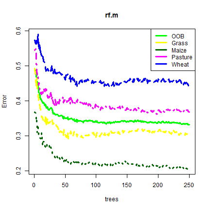
We can also plot the model object
cols <- c("green", "yellow", "darkgreen", "magenta", "blue")
plot(rf.m, col=cols, lwd=3)
legend("topright", col=cols , c("OOB", "Grass", "Maize","Pasture","Wheat"), lty=1, lwd=3)
There is a number of other tools to inspect the model. The “Variable Importance Plot” is an important tool that can be used with any regression-like model to determine the importance of individual variables.
varImpPlot(rf.m, main="")
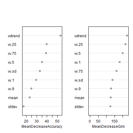
The plot shows each variable on the y-axis, and their importance on the x-axis. They are ordered top-to-bottom as most- to least-important. There are two plots namely:
- Mean decrease in accuracy. The lower the predictive performance of Random Forest due to the exclusion (randomization of the values, in fact) of particular single variable, the more important the variable is.
- Mean decrease in Gini estimates the contribution of each variable to achieve homogeneity in the groups created by the trees. Every time a variable is used to split the data (create a node), the Gini coefficient for the child nodes are estimated and compared to that of the data of the mother node. The Gini coefficient is a measure of homogeneity in the range of 0 (homogeneous) to 1 (heterogeneous). Variables that result in nodes with higher purity have a higher decrease in Gini coefficient.
You can also look at the raw data used to make the plot
importance(rf.m)
##             Grass      Maize    Pasture     Wheat MeanDecreaseAccuracy
## vv.1    11.722713 15.7477529 28.9026121  6.884381             34.46518
## vv.25   14.386066 27.6802409 27.8519828  7.919113             40.24326
## vv.5     8.999441 27.7065748 22.7955575 11.391493             36.41890
## vv.75   12.798359 29.7004243 12.9367550 10.152642             36.56193
## vv.9    15.597571 18.8046201  7.0462012  5.129844             26.40858
## vv.sd   27.062575 15.6677902 15.8759885  5.948151             33.37643
## vvtrend 29.580298  9.2572731 25.7870822 40.968655             52.63641
## mean    19.459227 -2.3950139 11.2794722 13.883768             23.72578
## stdev   15.799357  0.8795029  0.5913766 14.198168             17.47789
##         MeanDecreaseGini
## vv.1            179.8616
## vv.25           221.9055
## vv.5            200.7486
## vv.75           165.3855
## vv.9            121.0179
## vv.sd           136.9598
## vvtrend         224.4248
## mean            125.1059
## stdev           123.8068
Another good diagnostic tool is the partial-plot. It shows the response to a single variable (all other variables are kept at their original values).
partialPlot(rf.m, ref, "vvtrend", "Maize")
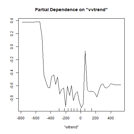
Like the variable importance plot, the partial plot can be computed for any regression-like (or classification) model; but there is not always a simple function available to quickly do it.
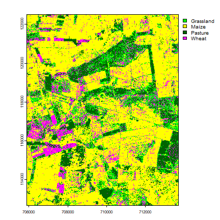
Model prediction
Now we use the model to predict the distribution of crops over the entire study region. This is the easy part.
rf.pred <- predict(img, rf.m)
rf.pred
## class       : SpatRaster
## dimensions  : 982, 783, 1  (nrow, ncol, nlyr)
## resolution  : 10, 10  (x, y)
## extent      : 705883.3, 713713.3, 112681.4, 122501.4  (xmin, xmax, ymin, ymax)
## coord. ref. : +proj=utm +zone=36 +datum=WGS84 +units=m +no_defs
## data source : memory
## names       : lyr.1
## min values  :     1
## max values  :     4
Make a map
rfp <- as.factor(rf.pred)
levels(rfp) <- c("Grassland", "Maize", "Pasture", "Wheat")
plot(rfp, col=c("green", "yellow", "darkgreen", "magenta"))
Post classifation improvements
TO DO: show and discuss the removal of noise
Model evaluation
It is important to evaluate predictive models. It allows comparison with alternative methods, and it can help establish some confidense in the predictions. Predictive models are generally evaluated with “cross-validation”. This is a technique in which the data are split in k folds. Each fold is held out once to evaluate the model created with the other folds. An evaluation statistic is computed for each fold, and averaged. Typically we use 5 or 10 fold cross-validation (do not use more folds).
Let’s make 5 “folds”. That is, each record is assinged to one of 5 groups
library(luna)
## Loading required package: httr
## Loading required package: readr
set.seed(530)
k <- kfold(ref, 5)
nrow(ref) / 5
## [1] 400
table(k)
## k
##   1   2   3   4   5
## 400 400 400 400 400
We now would need a loop to go over each fold, but here we just show the approach for a single fold.
Get training and testing samples
train <- ref[k != 1, ]
test  <- ref[k == 1, ]
Build a new model
rf <- randomForest(class~., data=train, ntree=250, importance=TRUE)
And use the model to make a prediction for the test data. Importantly, the model did not see the test data!
pred <- predict(rf, test)
And create a confusion matrix
conmat <- table(observed=test$class, predicted=pred)
conmat
##          predicted
## observed  Grass Maize Pasture Wheat
##   Grass      73    12      10    10
##   Maize       7    83       4    10
##   Pasture    17     4      51    15
##   Wheat      16    18      15    55
Compute one or more statistics
# overall accuracy
evaluate(conmat, "overall")
## [1] 0.655
# kappa
evaluate(conmat, "kappa")
## [1] 0.5386428
# user and producer accuracy
evaluate(conmat, "class")
##              Grass     Maize   Pasture     Wheat
## row-wise 0.6952381 0.7980769 0.5862069 0.5288462
## col-wise 0.6460177 0.7094017 0.6375000 0.6111111
Other algorithms
- Use the same data with another algorithm and compare the resuls.
References
Breiman, L., 2001. Random forests. Machine learning, 45(1), 5-32.
James, G., D. Witten, T. Hastie and R. Tibshirani, 2013. An Introduction to Statistical Learning. Springer.
This document was last generated on 2019-09-26.