Introduction to Google Earth Engine
by Aniruddah Ghosh
Introduction
This handbook describes how to utilize Google Earth Engine (GEE) to develop and implement analytics for cropland area mapping in Nigeria, using available dataset from various sources. GEE is a platform for analyzing large amounts of satellite data. It stores global satellite imagery from the past 40+ years in an organized fashion, facilitating large-scale data analysis. For a very quick introduction to GEE, watch this video.
This chapter is loosely based on contents of GEE developer guide and various presentations and code shared by Google Earth Engine developer team and others.
Before we start, let’s take a simple quiz. If you have not heard about any of the following “Vector”, “Raster”, “Landsat”, “Red-Near Infrared”, “NDVI” or “Reflectance”, consider first reading an introductory text on remote sensing. You can start with this website.
The methods discussed in this handbook can also be applied for similar applications in different regions.
Google Earth Engine Interface
Setting Up Google Earth Engine
The GEE platform is significantly different from traditional desktop remote sensing and GIS software. Therefore it might take some time to get adjusted with the platform. First of all, there are no desktop installers. The processing takes place in the cloud. You send your commands via an online interface with JavaScript. All you need is a web-browser. Google chrome is recommended, but you can also use Mozilla Firefox or Safari. GEE uses Google’s computational infrastructure for parallel processing, so it can process geospatial data much faster than an ordinary personal computer.
Next you need to create a developer account by filling the form. Its use is free for research, education, and nonprofit usage. After your account is approved, you can log in to the GEE interface. You can use Earth Engine either through the Explorer, a high-level point-and-click-only GUI or through the Playground, a more low-level IDE for writing custom scripts). It is also possible to use Python language to interact with the API, but that is beyond the scope of this handbook. Interested Python users can start here.
Optional reading If you never heard of cloud computing, there are a lot of materials available on how cloud computing works. Interested readers can start here.
GEE online code editor
After you login to your GEE account, you will see an interface like the following figure. You can write commands in JavaScript in the Code Editor and press run button to execute the commands. The key point is that the Code Editor runs in the browser and all the actual data processing is done on Google Servers in the background.
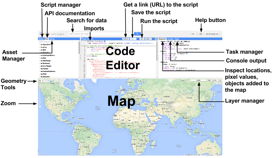
GEE code editor, source:https://developers.google.com
Optional reading More technical details about the Code Editor is available here.
Basic terminology
The two fundamental geographic data structures in Earth Engine are
Images are composed of georeferenced bands and a dictionary of properties. Features are composed of a geometry (point/line/polygons) and a dictionary of properties. Any collection is a bag of elements. A stack of images (e.g. an image time series) or multiple images with similar properties (e.g. all Landsat tiles) is handled by an ImageCollection (https://developers.google.com/earth-engine/ic_creating). A collection of features is handled by a FeatureCollection. Other fundamental data structures in Earth Engine include Dictionary, List, Array, Date, Number and String. If you are an R-user, you will find the following table useful to understand what we discussed above.
Using GEE online code editor
Brief introduction to Javascript
Javascript could be new to many of you. This guide will provide a quick introduction to the Earth Engine JavaScript API. You will learn how to create and print different data structures in GEE. Open your browser (Google Chrome preferred), go to Earth Engine Editor and start typing the following and click Run. Note that the code does not allow running single line or selected lines at a time. All the lines in the code editor will be executed at the same time. Therefore we will keep on adding/writing new lines and not remove the old ones.
print("Hello World!");
// variable
var season = "rain";
print("I like ", season);
// To comment use '//'
// print("Hello Mars!")
Basic Javascript data types
Most of these are declared with var.
Strings: Use single (or double) quotes to make a string.
Numbers: Numerics.
Lists: Defines with square brackets [ ] to store multiple objects.
Objects: Dictionaries of key: value pairs with curly brackets { }.
Now see one example for each of them
// Store a number in a variable.
var number = 10;
print('The answer is:', number);
// Use square brackets [] to make a list.
var numbers = [0, 1, 1, 2, 3, 5];
print('List of numbers:', numbers);
// Make a list of strings.
var strings = ['a', 'b', 'c', 'd', 'e'];
print('List of strings:', strings);
// Use curly brackets {} to make a dictionary of key:value pairs.
var object = {
  season: 'longrain',
  year: 2019,
  crops: ['maize', 'rice']
};
print('Dictionary:', object);
// Access dictionary items using square brackets.
print('Print year:', object['year']);
// Access dictionary items using dot notation.
print('Print stuff:', object.crops);
Functions
Functions are helpful to reuse to same lines of codes multiple times and improve readability of codes.
// Basic structure
var myFunction = function(parameter) {
  // do something
  statement;
  return statement;
};
Write an actual function
// Basic structure
var addnumber = function(number) {
  var newvalue =  number + 10
  return newvalue;
};
print(addnumber(20))
Earth Engine has a large number of in-built functions. You can find them in the Doc tab (upper left corner of the code editor).
// Make a sequence the hard way.
var eeList = ee.List([1, 2, 3, 4, 5]);
// Make a sequence the easy way!
var sequence = ee.List.sequence(1, 5);
print('Sequence:', sequence);
Applying functions multiple times
We can apply the functions on the list of numbers.
var sum1 = sequence.map(addnumber);
print("EE server computed objects ", sum1)
var sum2  = numbers.map(addnumber)
print("EE client computed objects ", sum2)
We will see the results are significantly different. sum1 values are
not human readable. This is related to Earth Engine internal working
mechanism and sooner or later you may come across this kind of
situations.
Optional To better understand what is happening here, you can read the section on client vs server.
Array
var array1 = ee.Array([1,2,3]) //1-D Array
print(array1.length());
var array2 = ee.Array([[1,2,3],[4,5,6]])
//2-D Array; use length() to return the lengths of each axis
print(array2.length());
var first = array2D.slice({axis: 0,start: 0,end: 1,step: 1});
print(first);
What is the closest R-object representation of array?
We can also create geographic objects.
Image
var image = ee.Image(1);
print(image);
Geometry and Feature
var point = ee.Geometry.Point([1.5, 1.5])
print(point)
var pointFeature = ee.Feature(point,
{name: 'mypoint', location: 'no-idea'})
print(pointFeature)
Optional reading For more details about the Earth Engine API, see the tutorials.
Working with a Landsat Image and ImageCollection
In this exercise, we show how you can search, find and visualize satellite data available through Google Earth Engine. We also describe different methods to mask clouds, create cloud free composites, calculate spectral indices, and finally export results. In this exercise we use Landsat data, but most of the examples can also be applied to any other satellite data available through Earth Engine. Learn more about the list of satellite data in Earth Engine Data Catalog.
Creating Feature and Feature Collection
Search, find and visualize image
To inspect any image (also called a scene) covering the area of interest (AOI), first we define the aoi (it can be a set of coordinates, points or polygons). We use the aoi location to filter the any image collection (e.g. all scenes captured by Landsat 8) and then use specific date ranges to limit the searches. In the following steps we show how to achieve this:
Search location: Search for ‘Ibadan’ in the Earth Engine playground search bar at the top and click the result to pan and zoom the map to Ibadan.
Use geometry tool: Use the geometry tools (upper right corner in the
map) to make a point in Ibadan (Important: exit the drawing tool when
you are finished). Name the resultant import point by clicking on
the import name (geometry by default).
Import satellite data: Search landsat 8 surface reflectance and
import the USGS Landsat 8 Surface Reflectance Tier 1
ImageCollection.
Spatial filter: Use the point you just created to find the data only over Ibadan
Temporal filter: Use a range of dates to confine the search results within a specific time period:
var collection = ee.ImageCollection('LANDSAT/LC08/C01/T1_SR');
// Construct start and end dates:
var start = ee.Date('2018-01-01');
var end = ee.Date('2018-12-31');
//Filter the Landsat 8 collection using the point and the dates
var filteredCollection = collection.filterBounds(point).filterDate(start, end);
// Inspect number of tiles returned after the search; we will use the one with more tiles
print(filteredCollection.size());
// Also Inspect one file
var image = filteredCollection.first();
print(image);
// print the band names
print(image.bandNames());
// Center the map on the image.
Map.centerObject(point, 9);
// Image display
Map.addLayer(image, {}, "Landsat surface reflectance");
// We specify visualization parameters in a JavaScript dictionary for better plots
var visParams = {
  bands: ['B4', 'B3', 'B2'],
  min: 0,
  max: 3000,
};
Map.addLayer(image, visParams, "Landsat surface reflectance");
Learn more about image information read the page on image information and metadata
We can sort the image collection by cloud cover. Often this is helpful find the least cloudy scene within a season.
var image = filteredCollection
              // Sort the collection by a metadata property.
              .sort('CLOUD_COVER')
              // Get the first image out of this collection.
              .first();
print('Least cloudy Landsat scene of the year:', image2);
Map.addLayer(image, visParams, "Landsat least cloudy image");
Exercise
Visualize false color composite image (NIR:red:green).
Create a dictionary of the image information and metadata properties including tile ID, resolution, projection, collection time and cloud cover.
Spectral Indices
Next we learn how to compute different vegetation indices and use thresholds to find specific land covers.
// Method 1: Using available function
var ndvi = image.normalizedDifference(['B5', 'B4']);
// Display the results
var ndviParams = {min: -1, max: 1, palette: ['blue', 'white', 'green']};
Map.addLayer(ndvi, ndviParams, 'NDVI');
// Method 2: Using band arithmetic
var nir = image.select('B5');
var red = image.select('B4');
var ndvi2 = nir.subtract(red).divide(nir.add(red)).rename('NDVI');
// Method 3: Using image expressions
var ndvi3 = image.expression(
    '(NIR - RED) / (NIR + RED)', {
      'NIR': image.select('B5'),
      'RED': image.select('B4')
});
Image expressions offer some flexibilities and are extremely useful for complicated indices such as EVI
We can use the NDVI layer and our knowledge of the study area and
try to find green areas.
// Create binary images from thresholds on NDVI.
// This threshold is excpected to detect green areas
var veg = ndvi.gt(0.4);
//Mask areas with the binary image
var green = veg.updateMask(veg);
// Define visualization parameters for the spectral indices.
var ndviViz = {min: -1, max: 1, palette: ['FF0000', '00FF00']};
Map.addLayer(green, ndviViz, 'vegetations');
Exercise
Use
imageto compute a spectral index for enhancing water (hint: NDWI = (green - NIR) / (green + NIR)) and built-up areas (hint: NDBI = (SWIR - NIR) / (SWIR + NIR)).Visualize the results of
NDWIandNDBI.Use a threshold to find the water and built locations.
Cloud Mask
So far we worked with the least cloudy image. We are using Landsat Surface Reflectance product for the analysis. This dataset is the atmospherically corrected surface reflectance from the Landsat 8 OLI/TIRS sensors. These images contain 5 visible and near-infrared (VNIR) bands and 2 short-wave infrared (SWIR) bands processed to orthorectified surface reflectance, and two thermal infrared (TIR) bands processed to orthorectified brightness temperature.
These data have been atmospherically corrected using LaSRC and includes a cloud, shadow, water and snow mask produced using CFMASK, as well as a per-pixel saturation mask.
Quality band, pixel_qa, contains Pixel quality attributes generated from the CFMASK algorithm. This is a bitmask and various quality information is bit-encoded in it. We use the following function to mask cloud and cloud shadows from the Landsat SR tiles.
/**
 * Function to mask clouds based on the pixel_qa band of Landsat 8 SR data.
 * @param {ee.Image} image input Landsat 8 SR image
 * @return {ee.Image} cloudmasked Landsat 8 image
 */
function maskL8sr(image) {
  // Bits 3 and 5 are cloud shadow and cloud, respectively.
  var cloudShadowBitMask = (1 << 3);
  var cloudsBitMask = (1 << 5);
  // Get the pixel QA band.
  var qa = image.select('pixel_qa');
  // Both flags should be set to zero, indicating clear conditions.
  var mask = qa.bitwiseAnd(cloudShadowBitMask).eq(0)
                 .and(qa.bitwiseAnd(cloudsBitMask).eq(0));
  return image.updateMask(mask);
}
We can apply this function for one image.
var image = filteredCollection.first();
var image_masked = maskL8sr(image);
Map.addLayer(image, visParams, "Landsat tile with cloud");
Map.addLayer(image_masked, visParams, "Landsat tile cloud masked");
We also use this function over entire collection and compare composites before and after cloud masking.
var maskedCollection = filteredCollection.map(maskL8sr);
Map.addLayer(filteredCollection.median(), visParams, "Landsat composite with cloud");
Map.addLayer(maskedCollection.median(), visParams, "Landsat composite cloud masked");
Any one satellite image may have various problems that can obscure the surface–a cloudy day, a plume of smoke–so creating a composite image can help give a better picture. By default, Earth Engine creates the composite using the most recent pixel in each case, but telling Earth Engine to choose the median value in the stack of possible pixel values can usually remove clouds, as long as you have enough images in the collection. Clouds have a high reflectance value, and shadows have a low reflectance value, so picking the median should give you a relatively cloudless composite image. Since we have Landsat images for growing season of each year and Landsat satellites take pictures of the same location about every two weeks, we can have multiple possible images to put together.
The tiles returned after cloud masking are not mosaiced or stacked, and
there are gaps in them after due to the masking of clouds. We first
combine
(reduce)
the tiles to create a single composite image representing one or
multiple statistics (e.g. mean, median, standard deviation, percentiles)
of the observations. This is same as [app] function in
(https://rdrr.io/github/rspatial/terra/man/app.html) function in
terra package.
// here we compute the following composites
// general structure: ImageCollection.reduce(ee.Reducer.Name(parameter));
// Mean
var mean = maskedCollection.reduce(ee.Reducer.mean());
//alternate: var mean = maskedCollection.mean();
// Median
var med = maskedCollection.reduce(ee.Reducer.median());
//alternate: var med = maskedCollection.median();
// Standard Deviation
var sd = maskedCollection.reduce(ee.Reducer.stdDev());
Exercise Visualize different composites we created above to learn more about their differences.
Once we are satisfied with the results of the percentile products, we can export the composites to Google Drive for future uses.
var CRS = 'EPSG:4326'; // Only if you want export in specific reference system
mean = mean.select(["B2_mean","B3_mean","B4_mean","B5_mean"])
Export.image.toDrive({
  image: mean,
  description: 'exporting-composite-to-drive',
  fileNamePrefix: 'ibadan_landsat_composite',
  folder: 'GEE_export', // Name of the Google Drive folder
  scale: 30,
  maxPixels: 1e13,
  crs: CRS
});
Exercise The following function can be used to mask cloud in USGS Landsat 8 Collection TOA Reflectance. Use this function to mask cloud in TOA product and recreate the workflow above.
// Simple Cloud Score
var maskCloudsTOA = function(image, th) {
  var scored = ee.Algorithms.Landsat.simpleCloudScore(image);
  //Specify cloud threshold (0-100)- lower number masks out more clouds
  var mask = scored.select(['cloud']).lte(th);
  //Make sure no band is just under zero
  var allBandsGT = image.reduce(ee.Reducer.min()).gt(-0.001);
  return image.updateMask(mask.and(allBandsGT));
};
var toa_dataset = ee.ImageCollection('LANDSAT/LC08/C01/T1_TOA');