Market access¶

Sebastian Palmas, CIMMYT

Introduction¶

Small scale farmers in developing countries are often characterised by their spatial dispersion. This factor gives them serious difficulties in accessing markets in urban centers where they can sell their goods or put them in a situation where they have to travel long distances in the uncertainty of finding a market for their production. Overall, this low market access may result in an uncertainty of income and failure in selling their products at a profit, or at a value enough to buy farm inputs such as fertilizer, pesticides, and improved technologies. Small-scale farmer thus enter poverty cycles as a consequence of poor market access (Barrett, 2008). The work by (Weiss, et al., 2018) highlighted the global disparities in accessibility relative to wealth, with sub-Saharan Africa being one of the areas with less access to markets.

Market access is (in part) a function of distance to market centers and transport infrastructure. Prices of outputs may be more volatile as the distance to market increases (Moctar et al., 2015) and inadequate road infrastructure increases the costs of tranportation for smallholder farmers (Obare, 2003)

The availability of open data sources such as Open Street Map gives researchers the possibility to capture market centers and infrastructure networks with unprecented detail and precision, specially in areas with low availability of data, such as sub-Saharan Africa.

In this example, we produce a market access raster in which each pixel in Tanzania is assigned a value that is the least accumulative cost of getting to a market center considering road access and land cover classes. The methodology in this script is meant to be completely replicable to other regions.

In this example, we use minutes per meter as the measure for travel cost.

Chapter requirements.¶

For this chapter you need the following R packages: terra, geodata, and reagro. See these instructions about installing these packages.

We first create a cost surface for transportation.

Transportation cost surface¶

Elevation and Slope¶

The first factor we will consider is slope. A slope is the rise or fall of the land surface and it is an important factor in determining travel costs. Movement speeds when traveling in flatter terrain are faster than in hillier or sloping areas.

For instance, when calculating cost distances, routes may avoid steep slopes that greatly reduce speed and instead calculate that the fastest route is through a flatter terrain, even if the actual distance may be longer than the route including slopes.

This slope layer will also be the template of all raster analysis. The rasterizing of road vector data, and the final prediction below will be matched to the extent and resolution of this slope layer.

We use the geodata package to download elevation data and then create a slope layer using the terra::slope function.

library(geodata)
tza_alt <- elevation_30s("Tanzania", path=".")
tza_slope <- terrain(tza_alt, "slope", unit="radians", neighbors=8)
plot(tza_slope, main="Slope")

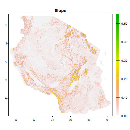
We use the slope layer obtained above to create a decay coefficient that governs how much the slope impacts the speed and that we will apply to each grid cell in the cost surface. We use a decay coefficient of 1.5.

decay <- 1.5
slope_cost <- exp( decay * tan(tza_slope) )
names(slope_cost) <- "slope_cost"

We will use the slope layer as template for the other rasters that we will create.

Roads¶

Open Street Map data¶

Ed: Perhaps this section should be a recipe on its own.

Road infrasturcture is a important predictive variable for market access and it is commonly used in market access protocols (e.g. World Bank, 2016). Transaction costs for remote rural households are high and, therefore, remoteness negatively affect the size of the agricultural surplus of these households market (Stifel and Minten, 2017).

One source of roads (and many other geospatial attributes) data is Open Street Map (OSM). OSM is a collaborative editable map of the world with an open data license (Open Data Commons Open Database License, ODbL) meaning that it is free to download as long as credit is given to OpenStreetMap and its contributors.

However, there are several cons of using OSM data. Because OSM depends on mapping volunteers, data quality and consistency is spotty. Places where there is a high concentration of mappers, the data can be very detailed and accurate (e.g. USA). However, areas such as sub-Saharan Africa, where there are less volunteers, the quality of data can be questionable and many areas can be without data coverage. A second con when using OSM is that the data is not authoritative. The data has not went through quality control and there is no statement of accuracy.

You can download the current OSM data in R using the osmdata package. But you can only download a relatively small amount of data in a single request, so typically you need to a number of requests for adjacent regions and then combine the results. Instead we use the road data that was preprocessed for the geodata package (and that may be a little bit out of date)

adm <- gadm("TZA", level = 1, path=".")
roads <- geodata::osm("Tanzania", "highways", ".")

The geometries in the OSM data is very detailed. Much more than we need in most analysis. We simplified the geometries to store less data and so that the example runs faster. You can also use the rmapshaper package for this type of tasks.

roads <- simplifyGeom(roads, tolerance=0.01)

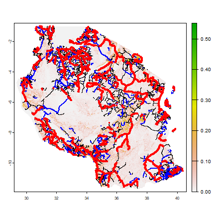
Now let’s have a look at the roads

plot(tza_slope)
lines(roads)
lines(roads[roads$highway == "secondary", ], lwd=2, col="blue")
lines(roads[roads$highway == "primary", ], lwd=4, col="red")

Road cost surface¶

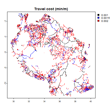
The road types have different moving speeds and, therefore, travel costs. Primary roads have faster speeds and lower travel costs than secondary and tertiary roads.

We rasterize the roads reflecting the travel speeds (in min/m) of moving through a cell by road (if there is one). We use the slope layer as template for the rasterization.

cfile <- "rdcost.tif"
roadtypes <- c("primary", "secondary", "tertiary")
if (!file.exists(cfile)) {
    i <- match(roads$highway, roadtypes)
    roads$speed <- c(0.001, 0.0015, 0.002)[i]
    rd_cost <- rasterize(roads, tza_slope, field=roads$speed, filename=cfile, wopt=list(names="slope_cost"), overwrite=TRUE)
    } else {
    # no need to repeat if we already have done this
    rd_cost <- rast(cfile)
}
# aggregate to improve visualization
a <- aggregate(rd_cost, 3, min, na.rm=TRUE)
plot(a, col=c("black", "blue", "red"), main="Travel cost (min/m)")

Land Cover¶

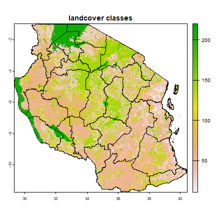
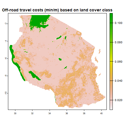
Environmental factors generally contribute to travel speeds off the transport network, such as land cover. Different types of land cover have different travel speeds depending on their “friction” or their ease of movement. For example, overland (on foot) movement through a closed forest is slower than movement through croplands or bare areas.

In this example, we use the the GLOBCOVER 2009 Version 2.3 land cover classification for Tanzania. More information about this classification can be gound in the ESA GlobCover portal. We included these data the agrodata package.

tza_lc <- agrodata::reagro_data("TZA_globcover")
plot(tza_lc, main = "landcover classes")
lines(adm)

As mentioned above, creating a travel cost surface depending on land cover requires an associated travel cost for each land class. See Weiss et al. (2018) for estimates of how long it takes individuals to traverse each land cover type. For now, we assign some travel cost values to the different land cover classes in Tanzania.

V a l u e	LandClass	Tra vel _sp eed
4 0	Closed to open (>15%) broadleaved evergreen or semi-deciduous forest (>5m)	0.0 4
5 0	Closed (>40%) broadleaved deciduous forest (>5m)	0.0 4
7 0	Closed (>40%) needleleaved evergreen forest (>5m)	0.0 4
1 6 0	Closed to open (>15%) broadleaved forest regularly flooded (semi-permanently or temporarily) - Fresh or brackish water	0.0 3
1 7 0	Closed (>40%) broadleaved forest or shrubland permanently flooded - Saline or brackish water	0.0 5
1 9 0	Artificial surfaces and associated areas (Urban areas >50%)	0.0 1
2 0 0	Bare areas	0.0 1
2 1 0	Water bodies	0.1 1
2 2 0	Permanent snow and ice	0.1 3

Create a reclassifiction matrix and use it to replace the landcover categories with travel-time estimates.

rc <- data.frame(from=unique(tza_lc)[,1], to=0.02)
rc$to[rc$from %in% c(190,200)] <- 0.01
rc$to[rc$from == 160] <- 0.03
rc$to[rc$from %in% c(40,50,70)] <- 0.04
rc$to[rc$from == 170] <- 0.05
rc$to[rc$from == 210] <- 0.11
rc$to[rc$from == 220] <- 0.13
#reclassifying
tza_lc_cost <- classify(tza_lc, rc)

Transform the land-cover based travel-time estimates to the raster geometry that we are using.

lcfname <- "lc_cost.tif"
if (!file.exists(lcfname)) {
  # first aggregate to about the same spatial resolution
  lc_cost <- aggregate(tza_lc_cost, 3, mean)
  # then resample
  lc_cost <- resample(lc_cost, tza_slope, filename=lcfname, wopt=list(names="lc_cost"), overwrite=TRUE)
} else {
  lc_cost <- rast(lcfname)
}

plot(lc_cost, main = "Off-road travel costs (min/m) based on land cover class")

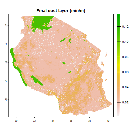
Combining travel costs¶

Now that we have all travel cost surfaces what we will use, we then need to combine them into a single travel cost layer that keeps only the minimum cost associated of moving though each grid cell. In this case, we combine the the road and off-road cost layers in a SpatRaster and apply the min function to obtain the minimum value in each grid cell. We multiply these values with the additional cost due to slopes.

# Combine the cost layers
all_cost <- c(rd_cost, lc_cost)
#getting the minimum value of each grid cell
cost <- min(all_cost, na.rm=TRUE)
cost <- cost * slope_cost
plot(cost, main="Final cost layer (min/m)")

Market access¶

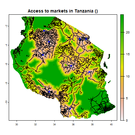
With the cost surface, we can compute market access by calculating the accumulated least cost surface from market locations. In other words, each pixel will have an associated cost of getting to a market center.

The minimum time to get to a city within a raster can be computed with the gdistance package using the accCost function.

When using least cost path analysis, the eight neighbors of a raster pixel are evaluated and the generated path moves to the cells with the smallest accumulated or cost value. This process is repeated multiple times until the source and destination are connected

We first need to install the package.

install.packages("gdistance")

We first need to create a transition matrix from the cost raster using the transition function. The transition objects are the central object in the gDistance package. They represent the weights given to each connection between grid cells (nodes).

In gdistance, conductance rather than resistance values are expected in the transition matrix (conductance is the inverse of resistance.) To create a transition object we need RasterLayer object with conductance values. We create if from a SpatRaster using the raster::raster method.

# Combine the cost layers
library(gdistance)
cost <- raster(cost)
conductance <- 1/cost
#Creating a transition object
tran <- transition(conductance, transitionFunction=mean, directions= 8)

Because the transition layer is based on a lon-lat projection and covers a large area, it is important to apply the geoCorrection function to adjust for for map distortion and diagonal connections between grid cells.

tran <- geoCorrection(tran, type="c")
## 'as(<dsCMatrix>, "dgTMatrix")' is deprecated.
## Use 'as(as(., "generalMatrix"), "TsparseMatrix")' instead.
## See help("Deprecated") and help("Matrix-deprecated").

With the transition object, we can now calculate access using the accCost function and supplying the coordinates from which to calulate.

In this code below, we make create a spatialpoint object with locations of some cities in Tanzania. In theory, cities locations can also be obtained using from OSM using osmdata. For, now we will supply some locations manually in form of a matrix.

lat=c(-6.17, -6.81, -5.02, -2.51, -3.65, -8.90, -3.34, -3.36, -10.67)
lon=c(35.74, 37.66, 32.80, 32.90, 33.42, 33.46, 37.34, 36.68, 35.64)
cities <- cbind(lon, lat)
spCities <- sp::SpatialPoints(cities)
#Estimating
Ac <- accCost(tran, fromCoords=spCities)

Bring the values back to a SpatRaster, and clamp the hightest values for better display

A <- rast(Ac) / 60
AA <- clamp(A, 0, 24) |> mask(tza_slope)
## Warning: [mask] CRS do not match
plot(AA, main="Access to markets in Tanzania ()")
lines(roads)
points(cities, col="blue", pch=20, cex=1.5)

References¶

Barrett, C.B., 2018. Smallholder market participation: Concepts and evidence from eastern and southern Africa. Food Policy 33(4):299-317. doi:10.1016/j.foodpol.2007.10.005.

Moctar, N., Elodie, M., Tristan, L., 2015. Maize Price Volatility, Does Market Remoteness Matter?. Policy Research working paper; no. WPS 7202. Washington, D.C.: World Bank Group. http://documents.worldbank.org/curated/en/132011468184160370/Maize-price-volatility-does-market-remoteness-matter

Obare, G.A., Omamo, S.W., Williams, J.C., B. 2003. Smallholder production structure and rural roads in Africa: the case of Nakuru District, Kenya. Agricultural Economics 28(3):245-254. doi:10.1111/j.1574-0862.2003.tb00141.x.

Stifel, D. and Minten, B., 2017,. Market Access, Well-being, and Nutrition: Evidence from Ethiopia. World Development 90:229-241. doi:10.1016/j.worlddev.2016.09.009.

Weiss, D.J., et al., 2018. A global map of travel time to cities to assess inequalities in accessibility in 2015. Nature 553:333-336. doi:10.1038/nature25181.

World Bank, 2016. Measuring rural access : using new technologies (English). Washington, D.C.: World Bank Group. http://documents.worldbank.org/curated/en/367391472117815229/Measuring-rural-access-using-new-technologies

Citation¶

Palmas, S., 2019. Spatial model of market access. In: Hijmans, R.J. and J. Chamberlin. Regional Agronomy: a pratical handbook. CIMMYT. https:/reagro.org/recipes/access.html