African maize trials
Here we use data that was also used in a paper by Lobell et al. Nonlinear heat effects on African maize as evidenced by historical yield trials.
Get the data
The data is on CIMMYT’s dataverse.
https://data.cimmyt.org/dataset.xhtml?persistentId=hdl:11529/10548190
The ID is “hdl:11529/10548190” and we can download the data with the “agro” package. This package is under development. You can install it like this (if need be):
if (!require(agro))  source("https://install-github.me/reagro/agro")
## Loading required package: agro
Now we can use the package to download the data
ff <- agro::get_data_from_uri("hdl:11529/10548190", ".")
ff
## [1] "./hdl_11529_10548190/EIL_site_latlon.zip.gz"
## [2] "./hdl_11529_10548190/maizedata.lobell.sep2011.csv.zip.gz"
We have two “gz” (GNU zip) files. We can g-unzip these
print(R.utils::gunzip(ff[1], remove=FALSE, overwrite=TRUE))
## [1] "hdl_11529_10548190/EIL_site_latlon.zip"
## attr(,"nbrOfBytes")
## [1] 3259
print(R.utils::gunzip(ff[2], remove=FALSE, overwrite=TRUE))
## [1] "hdl_11529_10548190/maizedata.lobell.sep2011.csv.zip"
## attr(,"nbrOfBytes")
## [1] 1153763
Now we have zip files that we can unzip
unzip("hdl_11529_10548190/EIL_site_latlon.zip")
unzip("hdl_11529_10548190/maizedata.lobell.sep2011.csv.zip")
Read the data
location <- read.csv('EIL_site_latlon.csv', stringsAsFactors=FALSE)
maize_all <- read.csv('maizedata.lobell.sep2011.csv', stringsAsFactors=FALSE)
Explore
head(location)
##   LocationID Country Location                      Region Latitude Longitude
## 1          5  ANGOLA   ANGOLA Eastern and Southern Africa     0.00      0.00
## 2          6  ANGOLA  CABINDA Eastern and Southern Africa    -5.60     12.20
## 3          7  ANGOLA   CACUSO Eastern and Southern Africa    -9.42     15.75
## 4          8  ANGOLA     CELA Eastern and Southern Africa   -11.42     15.12
## 5          9  ANGOLA  CHIANGA Eastern and Southern Africa   -12.73     15.83
## 6         10  ANGOLA  HUMPATA Eastern and Southern Africa   -15.03     13.43
##   ElevM
## 1     0
## 2    22
## 3  1067
## 4  1305
## 5  1693
## 6  1890
dim(maize_all)
## [1] 26142    37
maize <- maize_all[,c(1:9)]
maize$yield <- round(exp(maize$logYield), 1)
table(maize$Management)
##
## Drought Low N Low pH Maize Streak Virus
## 3244 2800 2032 353
## Optimal
## 17713
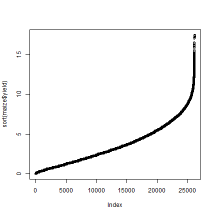
plot(sort(maize$yield))
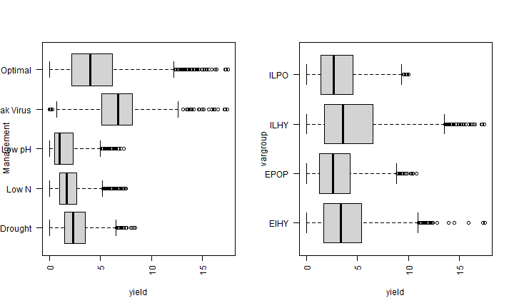
par(mfrow=c(1,2))
boxplot(yield ~ Management, data=maize, horizontal=TRUE, las=2)
boxplot(yield ~ vargroup, data=maize, horizontal=TRUE, las=2)
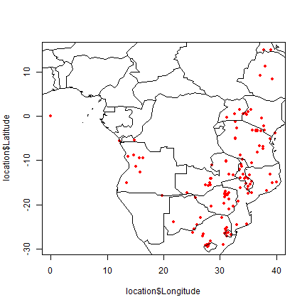
library(maptools)
## Loading required package: sp
## Checking rgeos availability: TRUE
## Please note that 'maptools' will be retired during 2023,
## plan transition at your earliest convenience;
## some functionality will be moved to 'sp'.
data(wrld_simpl)
plot(location$Longitude, location$Latitude, col="red", pch=20)
plot(wrld_simpl, add=TRUE)
Combine
d <- merge(location, maize, by.x="LocationID", by.y="sitecode")
dsub <- d[, c("yield","Longitude", "Latitude", "Management", "vargroup", "Country" )]
da <- aggregate(yield ~ ., data=dsub, median)
#da <- aggregate(d[,"yield",drop=FALSE], d[,-1], data=dsub, median)
da <- da[order(da[,1], da[,2]), ]
head(da)
##    Longitude Latitude Management vargroup Country yield
## 10     12.20    -5.60    Optimal     EIHY  ANGOLA  0.40
## 14     12.20    -5.60      Low N     EPOP  ANGOLA  0.30
## 16     12.20    -5.60     Low pH     EPOP  ANGOLA  0.85
## 31     12.20    -5.60     Low pH     ILPO  ANGOLA  0.30
## 40     12.20    -5.57    Optimal     ILPO  ANGOLA  0.00
## 4      13.43   -15.03    Optimal     EIHY  ANGOLA  4.50
table(da$Management, da$vargroup)
##
##                      EIHY EPOP ILHY ILPO
##   Drought              10   15    8    9
##   Low N                12   13    9   11
##   Low pH                7    9    7    8
##   Maize Streak Virus    1    2    1    1
##   Optimal              68   69   51   60
dopt <- da[da$Management=="Optimal", ]
Model
head(da)
## Longitude Latitude Management vargroup Country yield
## 10 12.20 -5.60 Optimal EIHY ANGOLA 0.40
## 14 12.20 -5.60 Low N EPOP ANGOLA 0.30
## 16 12.20 -5.60 Low pH EPOP ANGOLA 0.85
## 31 12.20 -5.60 Low pH ILPO ANGOLA 0.30
## 40 12.20 -5.57 Optimal ILPO ANGOLA 0.00
## 4 13.43 -15.03 Optimal EIHY ANGOLA 4.50
library(randomForest)
m <- randomForest(yield ~ Longitude + Latitude, data=da)
m
##
## Call:
## randomForest(formula = yield ~ Longitude + Latitude, data = da)
## Type of random forest: regression
## Number of trees: 500
## No. of variables tried at each split: 1
##
## Mean of squared residuals: 2.67184
## % Var explained: 40.28
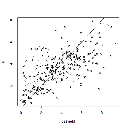
p = predict(m)
plot(da$yield, p)
abline(0,1)
library(raster)
e <- extent(c(-22, 60, -37, 24))
aoi <- raster(ext=e, res=1/6)
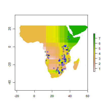
pp <- interpolate(aoi, m, xyNames=c('Longitude', 'Latitude'))
pp <- mask(pp, wrld_simpl)
plot(pp)
points(da$Longitude, da$Latitude, col="blue")
lon = init(aoi, "x")
lat = init(aoi, "y")
s <- stack(lon, lat)
names(s) <- c("Longitude", "Latitude")
p2 <- predict(s, m)
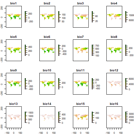
bio <- getData("worldclim", var="bio", res="10")
## Warning in getData("worldclim", var = "bio", res = "10"): getData will be removed in a future version of raster
## . Please use the geodata package instead
plot(bio)
e <- extract(bio, da[, c("Longitude", "Latitude")])
de <- cbind(da[,"yield",drop=FALSE], e)
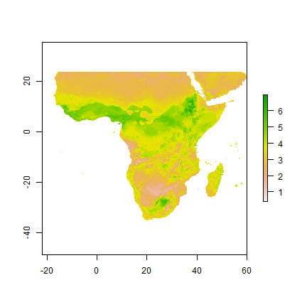
m <- randomForest(yield ~ ., data=de)
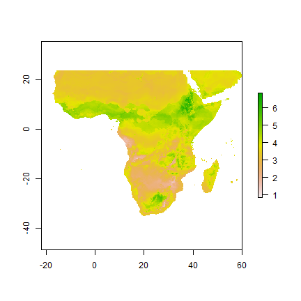
x <- predict(bio, m, ext=aoi)
plot(x)
de <- cbind(da, e)
head(de)
## Longitude Latitude Management vargroup Country yield bio1 bio2 bio3 bio4
## 10 12.20 -5.60 Optimal EIHY ANGOLA 0.40 248 75 55 1882
## 14 12.20 -5.60 Low N EPOP ANGOLA 0.30 248 75 55 1882
## 16 12.20 -5.60 Low pH EPOP ANGOLA 0.85 248 75 55 1882
## 31 12.20 -5.60 Low pH ILPO ANGOLA 0.30 248 75 55 1882
## 40 12.20 -5.57 Optimal ILPO ANGOLA 0.00 248 75 55 1882
## 4 13.43 -15.03 Optimal EIHY ANGOLA 4.50 173 133 65 1789
## bio5 bio6 bio7 bio8 bio9 bio10 bio11 bio12 bio13 bio14 bio15 bio16 bio17
## 10 309 173 136 265 219 265 219 912 170 0 83 477 2
## 14 309 173 136 265 219 265 219 912 170 0 83 477 2
## 16 309 173 136 265 219 265 219 912 170 0 83 477 2
## 31 309 173 136 265 219 265 219 912 170 0 83 477 2
## 40 309 173 136 265 219 265 219 912 170 0 83 477 2
## 4 265 63 202 182 147 188 144 796 169 0 89 425 0
## bio18 bio19
## 10 477 2
## 14 477 2
## 16 477 2
## 31 477 2
## 40 477 2
## 4 158 9
de$Country = NULL
de$Management <- as.factor(de$Management)
de$vargroup <- as.factor(de$vargroup)
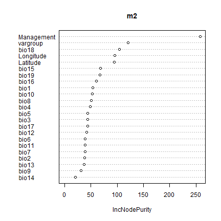
m2 <- randomForest(yield~., data=de)
m2
##
## Call:
## randomForest(formula = yield ~ ., data = de)
## Type of random forest: regression
## Number of trees: 500
## No. of variables tried at each split: 7
##
## Mean of squared residuals: 2.124513
## % Var explained: 52.51
varImpPlot(m2)
afbio <- crop(bio, s)
predictors <- stack(afbio, s)
df <- data.frame(Management="Optimal", vargroup="EPOP", stringsAsFactors = F)
df2 <- data.frame(Management="Optimal", vargroup="ILPO", stringsAsFactors = F)
#df <- data.frame(Management=5, vargroup=2)
pxd <- predict(predictors, m2, const=df2)
plot(pxd)
Now determine which vargroup performs best where, on average?
Do this for optimal and for drought?
when done, make it better…