Biofortified sweetpotato adoption
This case study will replicate the results from the article “Effect of Farmers’ Multidimensional Beliefs on Adoption of Biofortified Crops: Evidence from Sweetpotato in Tanzania”, by Shikuku et al. The purpose of this study is to see how farmers beliefs about orange-fleshed sweetpotato impacts their adoption of the variety.
This study uses data from both the baseline and endline surveys of the Marando Bora project, which can be found on dataverse here and here. The number of observations used for this study are those that were included in both the baseline and endline, a total of 434 households.
This case study will demonstrate how to clean and prepare data for analysis, to conduct summary statistics, and their estimation technique of inverse probability weighting and difference-in-differences (IPW-DID).
First we read in the data from both surveys:
The data
library(agro)
ffbase <- get_data_from_uri("https://data.cipotato.org/dataset.xhtml?persistentId=doi:10.21223/P3/QWFBBZ", ".")
head(ffbase)
## [1] "./doi_10.21223_P3_QWFBBZ/haconver.dta"
## [2] "./doi_10.21223_P3_QWFBBZ/mbase_questionnaire_20173001.xlsx"
## [3] "./doi_10.21223_P3_QWFBBZ/mbbase_dictionary_20173001.xls"
## [4] "./doi_10.21223_P3_QWFBBZ/mbbase_pg10_sold_gave_out_vines.dta"
## [5] "./doi_10.21223_P3_QWFBBZ/mbbase_pg10_vines_transaction.dta"
## [6] "./doi_10.21223_P3_QWFBBZ/mbbase_pg11_received_vines.dta"
ffend <- get_data_from_uri("https://data.cipotato.org/dataset.xhtml?persistentId=doi:10.21223/P3/ZQJNRS", ".")
head(ffend)
## [1] "./doi_10.21223_P3_ZQJNRS/haconver.dta"
## [2] "./doi_10.21223_P3_ZQJNRS/mbend_dictionary_20173001.xls"
## [3] "./doi_10.21223_P3_ZQJNRS/mbend_pg10_differences_of_MB_vines_from_others.dta"
## [4] "./doi_10.21223_P3_ZQJNRS/mbend_pg10_received_vines_elsewhere.dta"
## [5] "./doi_10.21223_P3_ZQJNRS/mbend_pg10_received_vines_marandobora.dta"
## [6] "./doi_10.21223_P3_ZQJNRS/mbend_pg11_pg13_sp_knowledge.dta"
First we read in the data from both surveys:
ff1 <- grep('\\.dta$', ffbase, value=TRUE)
#the data is stored as .dta from stata, so we need to use the package `readstata123`
library(readstata13)
x <- lapply(ff1, read.dta13, generate.factors=T, nonint.factors=T)
names(x) <- basename(ff1)
ff2 <- grep('\\.dta$', ffend, value=TRUE)
x2 <- lapply(ff2, read.dta13, generate.factors=T, nonint.factors=T)
names(x2) <- basename(ff2)
##Variables and Summary Statistics Next we will replicate summary statistics that are reported in table 1 and 2 of the paper. Table 1 provides an overview of outcomes/beliefs variables.The data source for these statistics is the endline survey, only including the observations that were also present in the baseline survey. Using the dictionary provided with the data, we can find which variables correlate to the questions that we are interestd in. We start with belief variables.
belief <- x2$`mbend_pg19_genderbased_attitude and perception_part1.dta`
#we only want observations below 627, since these are the ones that also appeared in the baseline.
belief <- belief[belief$hhid < 627,c(4, 9, 14:20, 34)]
colnames(belief) <- c("hhid", "health", "taste", "yield", "storability", "sweetness", "maturity", "child", "disease", "color")
#We need to switch the variables from the Linkert scale in which they were interviewed to 0-1 variables.
belief$health <- ifelse(belief$health == "Strongly agree" | belief$health == "Agree", 1, 0)
belief$taste <- ifelse(belief$taste == "Disagree" | belief$taste == "Strongly disagree", 1, 0)
belief$yield <- ifelse(belief$yield == "Strongly agree" | belief$yield == "Agree", 1, 0)
belief$storability <- ifelse(belief$storability == "Disagree" | belief$storability == "Strongly disagree", 1, 0)
belief$sweetness <- ifelse(belief$sweetness == "Disagree" | belief$sweetness == "Strongly disagree", 1, 0)
belief$child <- ifelse(belief$child == "Disagree" | belief$child == "Strongly disagree", 1, 0)
belief$disease <- ifelse(belief$disease == "Disagree" | belief$disease == "Strongly disagree",1, 0)
belief$maturity <- ifelse(belief$maturity == "Agree" | belief$maturity == "Strongly agree", 1, 0)
belief$color <- ifelse(belief$color == "Disagree" | belief$color == "Strongly disagree", 1, 0)
#mean and standard deviation of each variable
apply(belief[,-1], 2, mean)
##      health       taste       yield storability   sweetness    maturity
##   0.5783410   0.4170507   0.3709677   0.2764977   0.5092166   0.4170507
##       child     disease       color
##   0.5552995   0.3986175   0.6059908
apply(belief, 2, sd)
##        hhid      health       taste       yield storability   sweetness
## 168.6897229   0.4943945   0.4936404   0.4836213   0.4477820   0.5004920
##    maturity       child     disease       color
##   0.4936404   0.4975060   0.4901788   0.4892008
Next we will summarize outcome variables: household grew at least one OFSP variety, and change in proportion of OFSP roots of total production by household
sp <- x2$mbend_pg5_sweetpotato_production_table.dta
sp <- sp[sp$hhid < 627,c(4,12)]
colnames(sp) <- c("hhid", "OFSP")
sp$OFSP <- ifelse(sp$OFSP == "Yes", 1, 0)
#The data was recorded on a plot level, and we want household level--so we aggregate.
sp2 <- aggregate(sp$OFSP, list(sp$hhid), sum)
colnames(sp2) <- c("hhid", "OFSP")
sp2$OFSP[sp2$OFSP > 0] <- 1
summary(sp2$OFSP)
##    Min. 1st Qu.  Median    Mean 3rd Qu.    Max.
##  0.0000  0.0000  0.0000  0.3921  1.0000  1.0000
change <- x2$mbend_pg6_sp_production_cont.dta
change <- change[change$hhid < 627, c(4,7,10)]
#one of the responses was 50, which is an error, so it is converted to 10.
change$j27c[change$j27c>10] <- 10
change$change <- (change$j27c-change$j27f)/10
summary(change$change)
##     Min.  1st Qu.   Median     Mean  3rd Qu.     Max.
## -1.00000  0.00000  0.00000  0.03756  0.07500  1.00000
change <- change[,c(1,4)]
#add the outcome variables to the belief variables dataframe
allvar <- merge(sp2, change, by = "hhid")
allvar <- merge(allvar, belief, by = "hhid")
#Now we can
means <- round(apply(allvar[,-1], 2, mean, na.rm=T), 2)
knitr::kable(means)
x |
|
|---|---|
OFSP |
0.39 |
change |
0.04 |
health |
0.58 |
taste |
0.42 |
yield |
0.37 |
storability |
0.28 |
sweetness |
0.51 |
maturity |
0.42 |
child |
0.56 |
disease |
0.40 |
color |
0.61 |
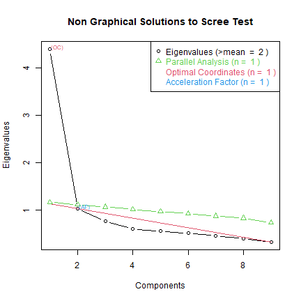
Following the methodology used in the paper, the authors next step is to use exploratory factor analysis to create a scree plot of Eigen values. The results of this analysis showed that tthere is a one factor solution. The authors further found that the variable maturity should not be retained for analysis.
library(nFactors)
## Warning: package 'nFactors' was built under R version 4.3.1
## Loading required package: lattice
##
## Attaching package: 'nFactors'
## The following object is masked from 'package:lattice':
##
##     parallel
belief <- belief[,-1]
ev <- eigen(cor(belief))
ap <- parallel(subject = nrow(belief), var=ncol(belief), rep=100, cent = .05)
nS <- nScree(x=ev$values, aparallel = ap$eigen$qevpea)
plotnScree(nS)
The authors also use a set of control variables, which are later used to generate propensity scores. These include household, farm, and market characteristics. Here we find each of the variables using the survey instrument and codesheet provided with the data, and combine the variables into a single data frame. We then add these variables to the previous belief variable dataframe.
dem <- x$mbbase_pg2_adult_demog.dta
demhhh <- dem[dem$D3=="Head",c(1, 3,5,8)]
colnames(demhhh) <- c("hhid", "sex", "age", "edu")
#hhhsex d2
demhhh$sex <- ifelse(demhhh$sex == "Male", 1, 0)
#hhhage 2009-d4
demhhh$age <- 2009-demhhh$age
#hhhedu above primary level d7
levels(demhhh$edu)<- c(0,0,0,0,0,0,0,0,1,1,1,1,1,1,1,1,1,1,1,1,1,1,1)
demhhh$edu <- as.numeric(as.character(demhhh$edu))
#infants number below five
dem2 <- x$mbbase_pg2_adult_demog.dta
dem2 <- dem2[,c(1,5)]
colnames(dem2) <- c("hhid", "age")
dem2$age <- 2009 - dem2$age
dem2$infants <- ifelse(dem2$age < 6, 1, 0)
#demhhh$infants <- aggregate(dem2$infants, list(dem2$hhid), sum)
#with the child data
child <- x$mbbase_pg3_child_demog.dta
child <- child[,c(1,6)]
colnames(child) <- c("hhid", "child")
child$child <- ifelse(child$child == "no infant", 0, 1)
child2 <- aggregate(child$child, list(child$hhid), sum)
colnames(child2) <- c("hhid", "child")
demhhh$infants <- child2$child
#noninfants number above five
dem2$noninfants <- ifelse(dem2$age > 5, 1, 0)
dem3 <- aggregate(dem2$noninfants, list(dem2$hhid), sum)
demhhh$noninfants <- dem3$x
#farmsize
farmsize <-x$`mbbase_pg5_crop production.dta`
farmsize <- farmsize[,c(1,4:6)]
farmsize$size <- farmsize$P02A + farmsize$P02B
demhhh$farmsize <- farmsize$size
#soldSP
#TODO: Find info from baseline, this is endline
sold <- x2$mbend_pg6_sp_production_cont.dta
sold <- sold[,c(4,11)]
colnames(sold) <- c("hhid", "sold")
sold$sold <- ifelse(sold$sold=="None at all", 0, 1)
#demhhh$sold <- sold$sold
#labour
labor <- x$mbbase_pg8_labour_and_credit.dta
labor <- labor[, c(1,5)]
colnames(labor) <- c("hhid", "labor")
labor$labor <- ifelse(labor$labor == "Only hired labor", 1, 0)
demhhh$labor <- labor$labor
#credit
credit <- x$mbbase_pg8_labour_and_credit.dta
credit <- credit[,c(1, 36, 37)]
colnames(credit) <- c("hhid", "applied", "received")
credit$credit <- ifelse(credit$applied == "Yes" & credit$received == "Yes", 1, 0)
demhhh$credit <- credit$credit
#region
mwanza <- x$mbbase_pg1_cover_page.dta$A01
mwanza <- ifelse(mwanza == "Mwanza", 1, 0)
demhhh$mwanza <- mwanza
mara <- x$mbbase_pg1_cover_page.dta$A01
mara <- ifelse(mara == "Mara", 1, 0)
demhhh$mara <- mara
#we only want the observations that were included in the allvar dataframe, which were the 434 observations from both surveys--so we use the argument all.x=T.
allvar <- merge(allvar,demhhh, all.x=T)
apply(allvar, 2, mean)
##         hhid         OFSP       change       health        taste        yield
## 271.35266821   0.39211137   0.03781903   0.58236659   0.41995360   0.37354988
##  storability    sweetness     maturity        child      disease        color
##   0.27842227   0.51276102   0.41995360   0.55916473   0.40139211   0.60788863
##          sex          age          edu      infants   noninfants     farmsize
##   0.77958237  47.04640371   0.08120650   1.36426914   6.02784223   2.61322494
##        labor       credit       mwanza         mara
##   0.32250580   0.31090487   0.61252900   0.38747100
##First stage: The authors use a methodology of inverse probability weighting and difference-in-differences (IPW-DID) to attempt to control for selection bias. Their first stage regression is to estimate the propensity scores, by regressing each of the belief variables on the control variables with a probit regression. Later, these propensity scores will be used as weights.
Here, because we regress different belief variables on the same set of explanatory variables, we can use a loop to run all the regressions at once, then store the coefficients (propensity scores) in a dataframe called “output”. This is demonstrated in table A1 in the appendix of the paper.
#empty dataframe in whcih to put the coefficients
output <- data.frame(matrix(NA, nrow=431, ncol=9))
#list of variables we use as independent variables in these regressions
k <- colnames(belief)
#Here we create a loop which puts the coefficients of each regression into the output dataframe.
for (i in seq_along(k)) {
  j <- k[i]
    fit <- glm(allvar[,j] ~ sex + age + edu + infants + noninfants + farmsize + labor + credit, family= binomial(link = "probit"), data = allvar)
  output[[i]] <- predict(fit, type = "response")
}
colnames(output) <- c("health.ate", "taste.ate", "yield.ate", "storability.ate", "sweetness.ate", "maturity.ate", "child.ate", "disease.ate", "color.ate")
Next, we use the propensity scores to determine weights for the regressions. According to the article, farmers in the treatment group have a weight of 1/p while farmers in the control group have a weight (1/1-p).
allvar$rownames <- rownames(allvar)
output$rownames <- rownames(output)
belief2 <- merge(allvar, output, by.x="rownames")
#for treatment: 1/output$health
#for control: 1/(1-output$health)
allvar$health.ate2 <- ifelse(belief2$health ==1, 1/belief2$health.ate, 1/(1-belief2$health.ate))
allvar$taste.ate2 <- ifelse(belief2$taste ==1, 1/belief2$taste.ate, 1/(1-belief2$taste.ate))
allvar$yield.ate2 <- ifelse(belief2$yield ==1, 1/belief2$yield.ate, 1/(1-belief2$yield.ate))
allvar$storability.ate2 <- ifelse(belief2$storability ==1, 1/belief2$storability.ate, 1/(1-belief2$storability.ate))
allvar$sweetness.ate2 <- ifelse(belief2$sweetness ==1, 1/belief2$sweetness.ate, 1/(1-belief2$sweetness.ate))
allvar$maturity.ate2 <- ifelse(belief2$maturity ==1, 1/belief2$maturity.ate, 1/(1-belief2$maturity.ate))
allvar$child.ate2 <- ifelse(belief2$child ==1, 1/belief2$child.ate, 1/(1-belief2$child.ate))
allvar$disease.ate2 <- ifelse(belief2$disease ==1, 1/belief2$disease.ate, 1/(1-belief2$disease.ate))
allvar$color.ate2 <- ifelse(belief2$color == 1, 1/belief2$color.ate, 1/(1-belief2$color.ate) )
##Second stage Now, that we have all the variables of interest, we can begin to run the regressions. The model used in the article is to regress the two outcome variables (whether the household grew OFSP, and the change in proportion grown) on the belief variables and control variables.
We begin with the regular, unweighted regressions.
fit <- lm(OFSP ~ health + yield + storability + sweetness + maturity + child + disease + color,  data=allvar)
summary(fit)
##
## Call:
## lm(formula = OFSP ~ health + yield + storability + sweetness +
##     maturity + child + disease + color, data = allvar)
##
## Residuals:
##      Min       1Q   Median       3Q      Max
## -0.80506 -0.24647 -0.08475  0.33700  0.93550
##
## Coefficients:
##             Estimate Std. Error t value Pr(>|t|)
## (Intercept)  0.08475    0.03806   2.227  0.02648 *
## health       0.07141    0.05284   1.352  0.17725
## yield        0.09751    0.05826   1.674  0.09494 .
## storability  0.14207    0.05398   2.632  0.00880 **
## sweetness    0.11410    0.05495   2.077  0.03844 *
## maturity     0.17662    0.05496   3.214  0.00141 **
## child        0.08675    0.06058   1.432  0.15284
## disease      0.05210    0.05299   0.983  0.32607
## color       -0.02025    0.04444  -0.456  0.64881
## ---
## Signif. codes:  0 '***' 0.001 '**' 0.01 '*' 0.05 '.' 0.1 ' ' 1
##
## Residual standard error: 0.4155 on 422 degrees of freedom
## Multiple R-squared:  0.2909, Adjusted R-squared:  0.2775
## F-statistic: 21.64 on 8 and 422 DF,  p-value: < 2.2e-16
fit2 <-lm(change ~ health + yield + storability + sweetness + maturity + child + disease + color,  data=allvar)
summary(fit2)
##
## Call:
## lm(formula = change ~ health + yield + storability + sweetness +
##     maturity + child + disease + color, data = allvar)
##
## Residuals:
##      Min       1Q   Median       3Q      Max
## -0.98809 -0.05504  0.01191  0.01605  0.89721
##
## Coefficients:
##              Estimate Std. Error t value Pr(>|t|)
## (Intercept) -0.011906   0.016834  -0.707    0.480
## health      -0.002961   0.023372  -0.127    0.899
## yield        0.037066   0.025770   1.438    0.151
## storability  0.018136   0.023874   0.760    0.448
## sweetness    0.031691   0.024303   1.304    0.193
## maturity     0.020895   0.024309   0.860    0.391
## child        0.024161   0.026794   0.902    0.368
## disease     -0.013103   0.023439  -0.559    0.576
## color       -0.001186   0.019657  -0.060    0.952
##
## Residual standard error: 0.1838 on 422 degrees of freedom
## Multiple R-squared:  0.0583, Adjusted R-squared:  0.04045
## F-statistic: 3.266 on 8 and 422 DF,  p-value: 0.001265
Next, we run the regressions with the weighted variables.
fitps <- lm(OFSP ~ health.ate2 + yield.ate2 + storability.ate2 + sweetness.ate2 + maturity.ate2 + child.ate2 + disease.ate2 + color.ate2, data=allvar)
summary(fitps)
##
## Call:
## lm(formula = OFSP ~ health.ate2 + yield.ate2 + storability.ate2 +
##     sweetness.ate2 + maturity.ate2 + child.ate2 + disease.ate2 +
##     color.ate2, data = allvar)
##
## Residuals:
##     Min      1Q  Median      3Q     Max
## -0.5577 -0.4002 -0.3184  0.5634  0.7539
##
## Coefficients:
##                   Estimate Std. Error t value Pr(>|t|)
## (Intercept)       0.462442   0.261316   1.770   0.0775 .
## health.ate2      -0.006833   0.068314  -0.100   0.9204
## yield.ate2        0.049037   0.041605   1.179   0.2392
## storability.ate2 -0.005629   0.024831  -0.227   0.8208
## sweetness.ate2    0.063815   0.091290   0.699   0.4849
## maturity.ate2     0.009049   0.054498   0.166   0.8682
## child.ate2       -0.091988   0.071768  -1.282   0.2006
## disease.ate2      0.014934   0.056264   0.265   0.7908
## color.ate2       -0.067502   0.053715  -1.257   0.2096
## ---
## Signif. codes:  0 '***' 0.001 '**' 0.01 '*' 0.05 '.' 0.1 ' ' 1
##
## Residual standard error: 0.4882 on 422 degrees of freedom
## Multiple R-squared:  0.02112,    Adjusted R-squared:  0.002565
## F-statistic: 1.138 on 8 and 422 DF,  p-value: 0.3362
fitps2 <- lm(change ~ health.ate2 + yield.ate2 + storability.ate2 + sweetness.ate2 + maturity.ate2 + child.ate2 + disease.ate2 + color.ate2, data=allvar)
summary(fitps2)
##
## Call:
## lm(formula = change ~ health.ate2 + yield.ate2 + storability.ate2 +
##     sweetness.ate2 + maturity.ate2 + child.ate2 + disease.ate2 +
##     color.ate2, data = allvar)
##
## Residuals:
##      Min       1Q   Median       3Q      Max
## -1.02410 -0.04682 -0.02885  0.00997  0.95248
##
## Coefficients:
##                   Estimate Std. Error t value Pr(>|t|)
## (Intercept)      -0.073847   0.100812  -0.733    0.464
## health.ate2       0.020822   0.026355   0.790    0.430
## yield.ate2       -0.001336   0.016051  -0.083    0.934
## storability.ate2  0.005615   0.009579   0.586    0.558
## sweetness.ate2    0.001235   0.035219   0.035    0.972
## maturity.ate2     0.033578   0.021024   1.597    0.111
## child.ate2       -0.004916   0.027687  -0.178    0.859
## disease.ate2     -0.001396   0.021706  -0.064    0.949
## color.ate2        0.002251   0.020723   0.109    0.914
##
## Residual standard error: 0.1883 on 422 degrees of freedom
## Multiple R-squared:  0.011,  Adjusted R-squared:  -0.007745
## F-statistic: 0.5869 on 8 and 422 DF,  p-value: 0.7889
This one has stat sig results, while the one above does not. I’m not sure what the difference is though!
healthps <- glm(health ~ sex + age + edu + infants + noninfants + farmsize + labor + credit, family= binomial(), data=allvar)
tasteps <- glm(taste ~ sex + age + edu + infants + noninfants + farmsize + labor + credit, family= binomial(), data=allvar)
yieldps <- glm(yield ~ sex + age + edu + infants + noninfants + farmsize + labor + credit, family= binomial(), data=allvar)
storabilityps <- glm(storability ~ sex + age + edu + infants + noninfants + farmsize + labor + credit, family= binomial(), data=allvar)
sweetnessps <- glm(sweetness ~ sex + age + edu + infants + noninfants + farmsize + labor + credit, family= binomial(), data=allvar)
maturityps <- glm(maturity ~ sex + age + edu + infants + noninfants + farmsize + labor + credit, family= binomial(), data=allvar)
childps <- glm(child ~ sex + age + edu + infants + noninfants + farmsize + labor + credit, family= binomial(), data=allvar)
diseaseps <- glm(disease ~ sex + age + edu + infants + noninfants + farmsize + labor + credit, family= binomial(), data=allvar)
colorps <- glm(color ~ sex + age + edu + infants + noninfants + farmsize + labor + credit, family= binomial(), data=allvar)
allvar$health.ate <-  predict(healthps, type="response")
allvar$taste.ate <- predict(tasteps, type = "response")
allvar$yield.ate <- predict(yieldps, type = "response")
allvar$storability.ate <- predict(storabilityps, type = "response")
allvar$sweetness.ate <- predict(sweetnessps, type = "response")
allvar$maturity.ate <- predict(maturityps, type = "response")
allvar$childps.ate <- predict(childps, type = "response")
allvar$disease.ate <- predict(diseaseps, type = "response")
allvar$color.ate <- predict(colorps, type = "response")
#for control: 1/(1-output$health)
allvar$health.ate2 <- ifelse(allvar$health ==1, 1/allvar$health.ate, 1/(1-allvar$health.ate))
allvar$taste.ate2 <- ifelse(allvar$taste ==1, 1/allvar$taste.ate, 1/(1-allvar$taste.ate))
allvar$yield.ate2 <- ifelse(allvar$yield ==1, 1/allvar$yield.ate, 1/(1-allvar$yield.ate))
allvar$storability.ate2 <- ifelse(allvar$storability ==1, 1/allvar$storability.ate, 1/(1-allvar$storability.ate))
allvar$sweetness.ate2 <- ifelse(allvar$sweetness ==1, 1/allvar$sweetness.ate, 1/(1-allvar$sweetness.ate))
allvar$maturity.ate2 <- ifelse(allvar$maturity ==1, 1/allvar$maturity.ate, 1/(1-allvar$maturity.ate))
allvar$child.ate2 <- ifelse(allvar$child ==1, 1/allvar$child.ate, 1/(1-allvar$child.ate))
allvar$disease.ate2 <- ifelse(allvar$disease ==1, 1/allvar$disease.ate, 1/(1-allvar$disease.ate))
allvar$color.ate2 <- ifelse(allvar$color == 1, 1/allvar$color.ate, 1/(1-allvar$color.ate))
fitps <- lm(OFSP ~ health.ate2 + yield.ate2 + storability.ate2 + sweetness.ate2 + maturity.ate2 + child.ate2 + disease.ate2 + color.ate2, data=allvar)
summary(fitps)
##
## Call:
## lm(formula = OFSP ~ health.ate2 + yield.ate2 + storability.ate2 +
##     sweetness.ate2 + maturity.ate2 + child.ate2 + disease.ate2 +
##     color.ate2, data = allvar)
##
## Residuals:
##     Min      1Q  Median      3Q     Max
## -0.8460 -0.3174 -0.1172  0.3867  0.9780
##
## Coefficients:
##                  Estimate Std. Error t value Pr(>|t|)
## (Intercept)       0.19724    0.22755   0.867 0.386537
## health.ate2      -0.11381    0.05961  -1.909 0.056893 .
## yield.ate2        0.06785    0.03718   1.825 0.068719 .
## storability.ate2  0.07487    0.02201   3.402 0.000733 ***
## sweetness.ate2   -0.03333    0.07757  -0.430 0.667604
## maturity.ate2     0.04194    0.04837   0.867 0.386390
## child.ate2        0.12446    0.03066   4.059 5.88e-05 ***
## disease.ate2      0.08514    0.05136   1.658 0.098155 .
## color.ate2       -0.01244    0.04752  -0.262 0.793566
## ---
## Signif. codes:  0 '***' 0.001 '**' 0.01 '*' 0.05 '.' 0.1 ' ' 1
##
## Residual standard error: 0.4305 on 422 degrees of freedom
## Multiple R-squared:  0.2388, Adjusted R-squared:  0.2244
## F-statistic: 16.55 on 8 and 422 DF,  p-value: < 2.2e-16
fitps2 <- lm(change ~ health.ate2 + yield.ate2 + storability.ate2 + sweetness.ate2 + maturity.ate2 + child.ate2 + disease.ate2 + color.ate2, data=allvar)
summary(fitps2)
##
## Call:
## lm(formula = change ~ health.ate2 + yield.ate2 + storability.ate2 +
##     sweetness.ate2 + maturity.ate2 + child.ate2 + disease.ate2 +
##     color.ate2, data = allvar)
##
## Residuals:
##      Min       1Q   Median       3Q      Max
## -0.99503 -0.05206 -0.00338  0.02556  0.92305
##
## Coefficients:
##                   Estimate Std. Error t value Pr(>|t|)
## (Intercept)       0.084406   0.097708   0.864    0.388
## health.ate2      -0.013544   0.025594  -0.529    0.597
## yield.ate2        0.013417   0.015965   0.840    0.401
## storability.ate2  0.011904   0.009450   1.260    0.208
## sweetness.ate2   -0.037830   0.033307  -1.136    0.257
## maturity.ate2     0.021336   0.020768   1.027    0.305
## child.ate2        0.020770   0.013166   1.577    0.115
## disease.ate2     -0.005121   0.022055  -0.232    0.817
## color.ate2       -0.011319   0.020403  -0.555    0.579
##
## Residual standard error: 0.1848 on 422 degrees of freedom
## Multiple R-squared:  0.04731,    Adjusted R-squared:  0.02924
## F-statistic: 2.619 on 8 and 422 DF,  p-value: 0.008305