Soil and Land Health
As part of the Africa RISING initiative, three sites in the Babati District of Tanzania were surveyed for various biophysical properties of the soil using the Land Degradation Surveillance Framework. At each 100 sq km site, 160 samples were taken. This case study will explore data from these sites, and map the spatial distribution of a few key variables. Some of the summary statistics were replicated from a powerpoint file that was included with the dataset.
The data come in two parts.They can be downloaded here and here. The first two sites, Long and Matufa, were part of a single dataset, and the third, Hallu, was a separate dataset. The files were not uploaded to dataverse in a consistent format. The files were in .csv, .tab, .xls, and .xlsx formats. For this reason, we need to call several functions to read in the data to R. Additionally, the excel files were uploaded to dataverse in a particularly messy way. Notes and comments from the researcher were included in the first rows of the tables, which create an extra difficulty when reading in the files to R–which we will correct for below.
We begin with analysis of the data from Long and Matufa, then combine with the datasets from Hallu.
First, we read in al the data. Since the first dataset is currently saved as both csv and excel files, so we upload the two formats separately and combine them into a single object with the append command.
library(agro)
f1 <- get_data_from_uri("https://doi.org/10.7910/DVN/CQLR9B", ".")
f2 <- get_data_from_uri("https://doi.org/10.7910/DVN/8JMMUZ", ".")
f1
##  [1] "./doi_10.7910_DVN_CQLR9B/02. Mafuta_Crop Nutrition Results for dataverse.xlsx"
##  [2] "./doi_10.7910_DVN_CQLR9B/03. Long Crop Nutrition Results for dataverse.xlsx"
##  [3] "./doi_10.7910_DVN_CQLR9B/04. Matufa LDPSA and CN for dataverse.xlsx"
##  [4] "./doi_10.7910_DVN_CQLR9B/05. Long LDPSA and CN for dataverse.xlsx"
##  [5] "./doi_10.7910_DVN_CQLR9B/06. LongMatufaMIRforDataverse.csv"
##  [6] "./doi_10.7910_DVN_CQLR9B/07. Matufa LDSF data raw for dataverse.csv"
##  [7] "./doi_10.7910_DVN_CQLR9B/08. Long_LDSF_data raw for dataverse .csv"
##  [8] "./doi_10.7910_DVN_CQLR9B/09. ldsf_description of codesv3_Matufa_Long.xlsx"
##  [9] "./doi_10.7910_DVN_CQLR9B/10. Matufa_Long Location Map.png"
## [10] "./doi_10.7910_DVN_CQLR9B/11. Winowiecki_Nov 2013_AfricaRISING Update Task1.2_sm.pptx"
f2
## [1] "./doi_10.7910_DVN_8JMMUZ/2 Hallu_Crop_Nutrition_Results.xls"
## [2] "./doi_10.7910_DVN_8JMMUZ/3 Hallu_Carbon_and_Nitrogen.csv"
## [3] "./doi_10.7910_DVN_8JMMUZ/5 Hallu_MIR.csv"
## [4] "./doi_10.7910_DVN_8JMMUZ/6 ICRAF_SSN_Hallu.csv"
## [5] "./doi_10.7910_DVN_8JMMUZ/7 Hallu_LDSF_data_raw.csv"
## [6] "./doi_10.7910_DVN_8JMMUZ/8 LDSF_description_of_codesv3.xlsx"
library(readxl)
ff <-  grep("\\.xlsx$", f1, value=TRUE)
ff2 <-  grep("\\.csv$", f1, value=TRUE)
x <- lapply(ff, read_xlsx)
## New names:
## New names:
## • `` -> `...2`
## • `` -> `...3`
## • `` -> `...4`
## • `` -> `...5`
## • `` -> `...6`
## • `` -> `...7`
## • `` -> `...8`
## • `` -> `...9`
## • `` -> `...10`
## • `` -> `...11`
## • `` -> `...12`
## • `` -> `...13`
## • `` -> `...14`
## • `` -> `...15`
## • `` -> `...16`
## • `` -> `...17`
## • `` -> `...18`
## • `` -> `...19`
## • `` -> `...20`
## • `` -> `...21`
## • `` -> `...22`
## • `` -> `...23`
## • `` -> `...24`
## • `` -> `...25`
## • `` -> `...26`
## • `` -> `...27`
x2 <- lapply(ff2, read.csv)
x3 <- append(x, x2)
In the Hallu dataset, four of the files were .tab, files, one was .xls, and one was .csv.
library(readxl)
library("readxl")
#ff3 <- list.files(datapath, pattern = "\\.xlsx$", full=T)
ff4 <- grep("\\.csv$", f2, value=TRUE)
ff5 <- grep("\\.xls$", f2, value=TRUE)
#x4 <- lapply(ff3, read_xlsx)
x5 <- lapply(ff4, read.csv)
x6 <- lapply(ff5, read_excel)
## New names:
## • `` -> `...3`
## • `` -> `...4`
## • `` -> `...5`
## • `` -> `...6`
## • `` -> `...7`
## • `` -> `...8`
## • `` -> `...9`
## • `` -> `...10`
## • `` -> `...11`
## • `` -> `...12`
## • `` -> `...13`
## • `` -> `...14`
## • `` -> `...15`
## • `` -> `...16`
## • `` -> `...17`
## • `` -> `...18`
## • `` -> `...19`
## • `` -> `...20`
#x7 <- append(x4, x5)
x7 <- x5
x8 <- append(x7, x6)
Summary Statistics
Now that we have read in the data, we show a few of the summary statistics graphically. The data did not come with a summary of variable names or description of the files. By reviewing the files that were included in the dataset, we can find which variables we need to create the following plots. To graph the plots, we use the package ggplot2, which has better data visualization graphics than base R.
Slope
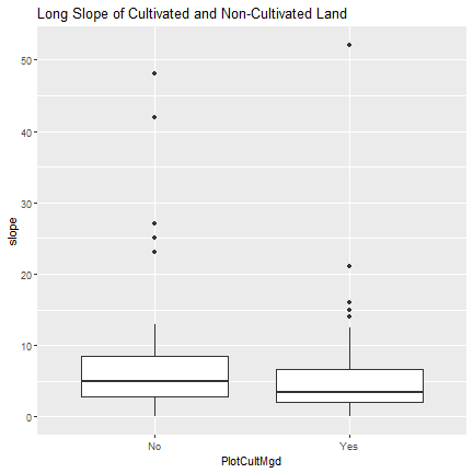
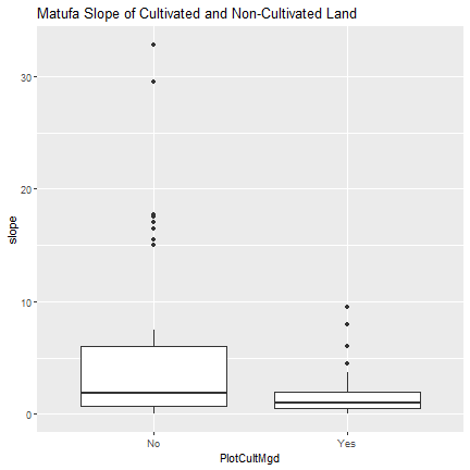
We will begin with a boxplot that shows the slope of land depending on whether or not the land is cultivated. Not surprisingly, it appears that on average plots that are cultivated are less sloped.
long <- x3[[8]]
#The variables of interest are "SlopeDn", "SlopeUp".
l.slope <- long[,c("SlopeUp", "SlopeDn", "PlotCultMgd")]
#We take the average of the two for each district.
l.slope$slope = (l.slope$SlopeDn + l.slope$SlopeDn)/2
library(ggplot2)
#long boxplot
 ggplot(l.slope, aes(x=PlotCultMgd, y = slope)) +
      geom_boxplot() +
   ggtitle("Long Slope of Cultivated and Non-Cultivated Land")
#We use the same code as we did above for long
matufa <- x3[[7]]
m.slope <- matufa[,c("SlopeUp", "SlopeDn", "PlotCultMgd")]
m.slope$slope <- (m.slope$SlopeUp + m.slope$SlopeDn)/2
#matufa boxplot
 ggplot(m.slope, aes(x=PlotCultMgd, y = slope)) +
      geom_boxplot() +
   ggtitle("Matufa Slope of Cultivated and Non-Cultivated Land")
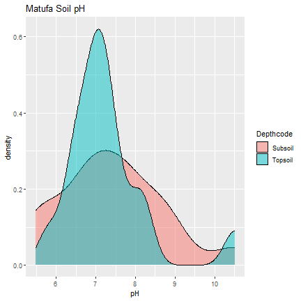
Soil pH
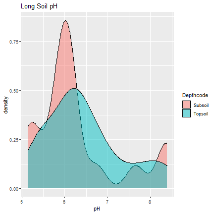
Next, we look at soil pH, using density plots to see the distribution of soil pH across plots. The excel graph for Long was “messy”, so we have to delete some of the rows to clean it up.
long_soil <-x3[[2]]
#delete the first ten rows
long_ph <- long_soil[-c(1:10),c(10:11)]
colnames(long_ph) <- c("Depthcode", "pH")
long_ph$pH <- as.numeric(long_ph$pH)
#we differentiate between subsoil and topsoil, and use alpha=.5 to be able to see both at once
ggplot(long_ph, aes(pH, fill=Depthcode)) +
  geom_density(alpha=.5) +
  ggtitle("Long Soil pH")
matufa_soil <- x3[[1]]
ggplot(matufa_soil, aes(pH, fill=Depthcode)) +
  geom_density(alpha = .5) +
  ggtitle("Matufa Soil pH")
Now we will graph the topsoil in all 3 districts together, adding the data from Hallu.
hallu_soil <-x8[[6]]
## Error in x8[[6]]: subscript out of bounds
#The excel graph was "messy", so we have to delete some of the rows to clean it up
hallu_ph <- hallu_soil[-c(1:7),c(3:4)]
## Error in eval(expr, envir, enclos): object 'hallu_soil' not found
colnames(hallu_ph) <- c("Depthcode", "pH")
## Error: object 'hallu_ph' not found
hallu_ph$pH <- as.numeric(hallu_ph$pH)
## Error in eval(expr, envir, enclos): object 'hallu_ph' not found
matufa_ph <- matufa_soil[,c(9:10)]
matufa_ph$District <- "matufa"
hallu_ph$District <- "hallu"
## Error: object 'hallu_ph' not found
long_ph$District <- "long"
all <- rbind(long_ph, hallu_ph, matufa_ph)
## Error in eval(expr, envir, enclos): object 'hallu_ph' not found
all <- all[all$Depthcode=="Topsoil" | all$Depthcode=="Top Soil",]
## Error in all$Depthcode: object of type 'builtin' is not subsettable
ggplot(all, aes(pH, fill=District)) +
  geom_density(alpha=.5) +
  ggtitle("TopSoil pH")
## Error in `ggplot()`:
## ! `data` cannot be a function.
## ℹ Have you misspelled the `data` argument in `ggplot()`
Spatial Distribution of sites
At this point, we will look at the data from all three sites. Lat/long
data was included in the dataset for the location of each of the sites
where soil samples were taken. Here we plot the sites against a backdrop
of the district in Tanzania, Babati. We get the map of Babati from GADM,
a database of geographic boundaries, using the function getData. To
do this, we need to upload a number of additional packages.
library(maptools)
## Loading required package: sp
## Checking rgeos availability: TRUE
## Please note that 'maptools' will be retired during 2023,
## plan transition at your earliest convenience;
## some functionality will be moved to 'sp'.
library(raster)
library(plyr)
library(rgdal)
## Please note that rgdal will be retired during 2023,
## plan transition to sf/stars/terra functions using GDAL and PROJ
## at your earliest convenience.
## See https://r-spatial.org/r/2022/04/12/evolution.html and https://github.com/r-spatial/evolution
## rgdal: version: 1.6-6, (SVN revision 1201)
## Geospatial Data Abstraction Library extensions to R successfully loaded
## Loaded GDAL runtime: GDAL 3.6.2, released 2023/01/02
## Path to GDAL shared files: C:/soft/R/R-4.3.0/library/rgdal/gdal
##  GDAL does not use iconv for recoding strings.
## GDAL binary built with GEOS: TRUE
## Loaded PROJ runtime: Rel. 9.2.0, March 1st, 2023, [PJ_VERSION: 920]
## Path to PROJ shared files: C:/soft/R/R-4.3.0/library/rgdal/proj
## PROJ CDN enabled: FALSE
## Linking to sp version:1.6-0
## To mute warnings of possible GDAL/OSR exportToProj4() degradation,
## use options("rgdal_show_exportToProj4_warnings"="none") before loading sp or rgdal.
#get boundaries of Tanzania, at district level
Tanz <- getData("GADM", country="TZ", level=2)
## Warning in getData("GADM", country = "TZ", level = 2): getData will be removed in a future version of raster
## . Please use the geodata package instead
#get the lat/long data
longlat1<- cbind(long$Longitude, long$Latitude, long$Altitude)
longlat2 <- cbind(matufa$Longitude, matufa$Latitude, matufa$Altitude)
hallu <- x8[[5]]
longlat3 <- cbind(hallu$Longitude, hallu$Latitude, hallu$Altitude)
## Warning: Unknown or uninitialised column: `Longitude`.
## Warning: Unknown or uninitialised column: `Latitude`.
## Warning: Unknown or uninitialised column: `Altitude`.
#convert to spatialpoints
ptslong <- SpatialPoints(longlat1)
ptsmatufa <- SpatialPoints(longlat2)
ptshallu <- SpatialPoints(longlat3)
## Error in (function (classes, fdef, mtable) : unable to find an inherited method for function 'coordinates' for signature '"NULL"'
#We only want the polygons in Tanzania for Babati, not the entire country
Babati <- Tanz[Tanz@data$NAME_2=="Babati",]
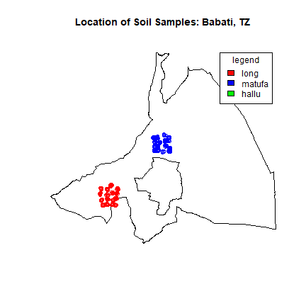
Now we can actually plot the data. We use different colors for each district. The polygon inside Babati is the urban district of Babati. We can see both clusters represent the 160 random soil samples.
#to plot all the points on map of Babati
plot(Babati, main="Location of Soil Samples: Babati, TZ")
points(ptslong, col="red")
points(ptsmatufa, col="blue")
points(ptshallu, col="green")
## Error in eval(expr, envir, enclos): object 'ptshallu' not found
legend("topright", inset=.05, title="legend", c("long", "matufa", "hallu"), fill=c("red", "blue", "green"))
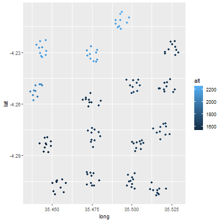
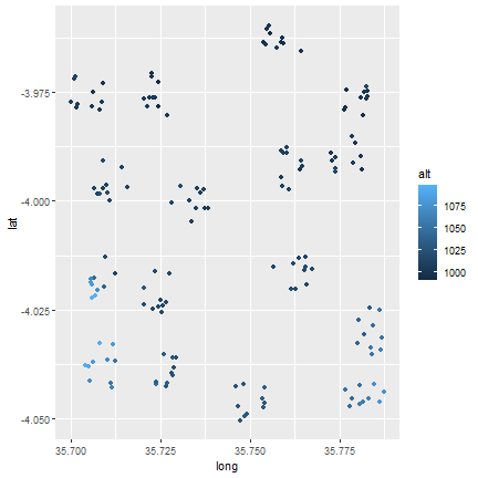
Next, can plot the altitude to get an idea of the spatial distribution of the altitude across the sites. Since we do the same set of commands three times, we can create a loop to simplify the code a bit.
l <- list(longlat1, longlat2, longlat3)
names(l) <- c("Long", "Matufa", "Hallu")
for (i in l) {
  j <- as.data.frame(i)
  colnames(j) <- c("long", "lat", "alt")
  print(ggplot(j, aes(x=long, y=lat)) +
  geom_point(aes(fill=alt, color=alt)))
}
## Error in names(x) <- value: 'names' attribute [3] must be the same length as the vector [0]
#TODO: Make titles on graphs