Effect of nitrogen and plant density on upland rice
1. Introduction
This case study shows how to investigate the effects of different levels of nitrogen, plant density on the growth and yield of interspecific rice varities.
We follow the analysis in a study by Oikeh et al (2009) entitled “Responses of upland NERICA rice varieties to nitrogen and plant density”. It was published in the Archives of Agronomy and Soil Science. You can access the article here (it is behind a paywall). The data was made avaliable on AfricaRice Dataverse and can be downloaded. But only one year data is available (2006) while the study describes two years.
The experiment took place at the IITA/WARDA Station, Cotonou, Benin, during the rainy season of 2006.
The treatments in this experimental study are four rice varities, three “New Rice for Africa (NERICA)” types and one check (WAB 450-I-B-P-38-HB (NERICA 1), WAB 450-I-B-P-20-HB (NERICA 2), WAB 450-I-B-P-91-HB (NERICA 4), WAB 56-50); four levels of nitrogen (0, 30, 60 and 120 kg/ha, applied as urea); and three planting distance (30 × 30 cm, 20 × 20 cm, and 25 × 5 cm). The seed was drilled for the 25 × 5 cm planting distance and dibbled for the other two distances.
Here we analyze the observations of grain yield and plant height. We note that the results are different here from those reported in the paper. (Already emailed to author)
2. Get the data
library(agro)
ff <- get_data_from_uri("https://dataverse.harvard.edu/dataset.xhtml?persistentId=hdl:1902.1/18485", ".")
ff
## [1] "./hdl_1902.1_18485/Responses of upland NERICA rice varieties to nitrogen and plant density.xlsx"
The data is provided as an excel spreadsheet. These files can be read with the ‘readxl’ package. The file has a single sheet. It is poorly organized as the first rows of the sheet are metadata (general and treatment information), and the actual data starts on row 23. Good practise would have been to use two different sheets. We read the sheet by skipping the first 22 rows.
library(readxl)
d <- read_xlsx(ff, skip = 22)
## New names:
## • `Number of lines` -> `Number of lines...19`
## • `Number of lines` -> `Number of lines...31`
We get a warning because the variable name “Number of lines” occurs twice.
We are going to analyze plant height and grain yield (dry matter). The variable names are a bit long, so we change them to someting more practical.
colnames(d)[c(12, 30)]
## [1] "Height Mat (cm)"
## [2] "Adjusted 14% grains dry weight kg/ha"
colnames(d)[12] <- "height"
colnames(d)[30] <- "yield"
colnames(d)[c(12, 30)]
## [1] "height" "yield"
Also, we express yield in ton (1000 kg) / ha instead of in kg/ha
d$yield <- d$yield / 1000
Another common mistake we find in these data is the use of integer codes for treatment instead of a clear label. We fix that.
table(d$N)
##
##  0  1  2  3
## 36 36 36 36
d$N <- c(0,30,60,120)[d$N + 1]
table(d$N)
##
##   0  30  60 120
##  36  36  36  36
table(d$V)
##
##  1  2  3  4
## 36 36 36 36
d$V <- c("Nerica 1", "Nerica 2", "Nerica 3", "WAB 56-104")[d$V]
table(d$V)
##
##   Nerica 1   Nerica 2   Nerica 3 WAB 56-104
##         36         36         36         36
table(d$D)
##
##  1  2  3
## 48 48 48
d$D <- c("dib30", "dib20", "drill")[d$D]
table(d$D)
##
## dib20 dib30 drill
##    48    48    48
3. Explore data
ANOVA
Here we reproduce the ANOVA for plant height as influenced by Varieties (V), Nitrogen (N) and plant density (D) levels. As only one year data is available online, the “year” factor is omited here.
First transform “D” and “v” from character to categorical variables.
d$D <- as.factor(d$D)
d$V <- as.factor(d$V)
Specify a linear model with all effects and interactions and a quadratic effect of nitrogen; and do the analysis of variance. Here is some more info on Linear Models, ANOVA, GLMs and Mixed-Effects models in R.
m <- lm(height ~ N * D * V + I(N^2), data = d)
anova(m)
## Analysis of Variance Table
##
## Response: height
##            Df Sum Sq Mean Sq  F value    Pr(>F)
## N           1 3331.3  3331.3 122.9677 < 2.2e-16 ***
## D           2 2933.7  1466.9  54.1465 < 2.2e-16 ***
## V           3  421.6   140.5   5.1875  0.002105 **
## I(N^2)      1   92.7    92.7   3.4223  0.066801 .
## N:D         2   44.8    22.4   0.8268  0.439949
## N:V         3   44.0    14.7   0.5410  0.655118
## D:V         6  277.8    46.3   1.7092  0.124622
## N:D:V       6  366.8    61.1   2.2569  0.042452 *
## Residuals 119 3223.8    27.1
## ---
## Signif. codes:  0 '***' 0.001 '**' 0.01 '*' 0.05 '.' 0.1 ' ' 1
Plots
Figure 2 shows a bar plot for the influence of N on plant height.
A clear repsonse to N is apparent from the boxplot of rice height vs. N level
boxplot(height ~ N, data = d)
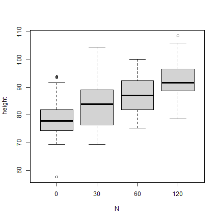
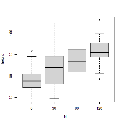
The boxplot shows that there are outliers. Here is a way to remove these. Here is some more info on outlier detection and removal with R.
nols.2q <- function(x, var="height") {
    m <- median(x[[var]], na.rm=TRUE)
    r <- quantile(x[[var]], c(0.25, 0.75), na.rm=TRUE)
    r <- 2 * diff(r)
    i <- which(abs(x[[var]] - m) < r)
    x[i,]
}
Nlev <- unique(d$N)
out <- vector(length=length(Nlev), mode="list")
for (i in 1:length(Nlev)) {
  dd <- d[d$N == Nlev[i], ]
  out[[i]] <- nols.2q(dd, var="height")
}
dd <- do.call(rbind, out)
boxplot(height ~ N, data = dd)
Calculate the mean height for each nitrogen level without outliers
height_N <- aggregate(dd[, 'height', drop=FALSE], dd[, 'N', drop=FALSE], mean)
# Caculate standard errors (can also use aggregate function here)
height_N_sem <- tapply(d$height, d$N, sd) / sqrt(tapply(d$height, d$N, length))
# Make the bar plot
xp <- barplot(height~N, data=height_N, xlab="Nitrogen (kg/ha)", ylab="Plant height (cm)", ylim = c(0,100), space = 1)
box(bty="l")
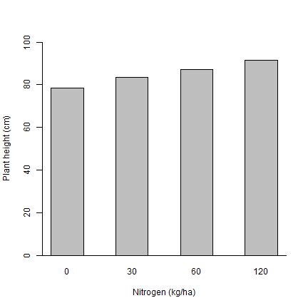
# Add error bars
arrows (p, (height_N$height - height_N_sem), p, (height_N$height + height_N_sem), code = 3, angle = 90, length = 0.05)
## Error in eval(expr, envir, enclos): object 'p' not found
3.3. Influence of N application on grain yield
This is for Table 2
# Caculate mean grain yield for each N level
Yield_N <- aggregate(d[, "yield", drop=FALSE], d[, "N", drop=FALSE], mean)
# Perform the simple linear regression between yield and nitrogen level using the lm function
Nyield_analysis <- lm (yield ~ as.factor(N), data = d)
Compute Tukey Honest Significant Differences to check if there are significant difference between each level.
TukeyHSD(aov(Nyield_analysis))
##   Tukey multiple comparisons of means
##     95% family-wise confidence level
##
## Fit: aov(formula = Nyield_analysis)
##
## $`as.factor(N)`
##               diff        lwr       upr     p adj
## 30-0    0.14321881 -0.1096697 0.3961073 0.4568035
## 60-0    0.12223646 -0.1306520 0.3751249 0.5918919
## 120-0   0.02537514 -0.2275133 0.2782636 0.9937516
## 60-30  -0.02098235 -0.2738708 0.2319061 0.9964382
## 120-30 -0.11784367 -0.3707322 0.1350448 0.6205144
## 120-60 -0.09686132 -0.3497498 0.1560272 0.7519834
This suggests that there is no significant difference between each N level on yield.
3.4 Yield vs. Nitrogen by variety
Plotted in a different shape for Figure 3
Aggregate data by Nitrogen and Variety group and caculate the mean yield for each group
yNV <- aggregate(d[, "yield", drop=FALSE], d[, c("N","V"), drop=FALSE], mean)
cols <- c("red", "blue", "orange", "black")
plot(yNV$N, yNV$yield, xlab = "N (kg/ha)", ylab = "Grain yield (ton/ha)", pch = c(15, 16, 17, 18)[yNV$V], col=cols[yNV$V], ylim=c(200, 1000), cex=1.5)
legend ("bottomleft", legend = levels(yNV$V), pch = c(15:18), col=cols, horiz=TRUE, cex=1.25)