Water use efficiency in potato
Introduction
This case study replicates results from the study “Effect of partial root-zone drying irrigation timing on potato tuber yield and water use efficiency” by Yactayo et al (2013), which was published in Agricultral Water Management. You can access the article on-line (it is behind a paywall). The data can be downloaded from the CIP dataverse.
Partial root-zone drying (PRD) is an irrigation technique has been can improve the water use efficiency (WUE) without reducting crop yields. This study investigated the effect of the level and timing of water restriction. They testd two PRD treatments with 25% (PRD25) and 50% (PRD50) of total water used in full irrigation (FI, as control), and a deficit irrigation treatment with 50% of water restriction (DI50). Two water restriction initiation timings were tested at: 6 weeks (WRIT6w) and 8 weeks (WRIT8w) after planting.
Data
library(agro)
ff <- get_data_from_uri("https://doi.org/10.21223/P3/MIVGMU", ".")
ff
## [1] "./doi_10.21223_P3_MIVGMU/Datos Yactayo et al_2013 (PRD).xlsx"
## [2] "./doi_10.21223_P3_MIVGMU/Dictionary_OA_Yactayo.xlsx"
The data is in an Excel spreadsheet with several sheets. The other Excel file has the data dictionary. Here we use the ‘openxlsx’ package to read the data.
library(openxlsx)
## Warning: package 'openxlsx' was built under R version 4.3.1
getSheetNames(ff[1])
## [1] "Read me"      "RWC"          "Chl SPAD"     "OP"           "TY"
## [6] "WUE"          "CWD"          "Weather data"
Read the sheets for tuber yield (TY), water use efficiency (WUE), and crop water demand (CWD)
# tuber yield
ty <- read.xlsx(ff[1], sheet="TY")
# water use efficiency
wue <- read.xlsx(ff[1], sheet = "WUE", startRow = 6)
# crop water demand
cwd <- read.xlsx(ff[1], sheet = "CWD", startRow = 2)
We also read relative water content (RWC). That is an ugly sheet as it has two tables in one sheet, one above the other. After some trial and error, we can read the two tables like this.
rwc6 <- read.xlsx(ff[1], sheet = "RWC", rows=2:20)
rwc8 <- read.xlsx(ff[1], sheet = "RWC", startRow=22)
Analyze data
Table 1
F-value of ANOVA of tuber yield and irrigation water use efficiency (WUE). Water restriction initiation timing at 6 (WRIT6w) and 8 (WRIT8w) weeks after planting. IT = irrigation treatment.
F-value of ANOVA of tuber yield for different water restriction initiation time at 6 (WRIT6w) and 8 weeks (WRIT8w) after planting.
Separate tuber yield data for two groups WRIT6w and WRIT8w as in the study
ty_WRIT6W <- ty[ty$T == "WRIT6w", ]
colnames(ty_WRIT6W)[4] <- "TY"
ty_WRIT8W <- ty[ty$T == "WRIT8w", ]
colnames(ty_WRIT8W)[4] <- "TY"
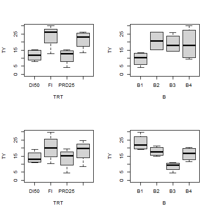
Some visual inspection of the distribution of the values is always a good start to see if everything looks reasonable.
par(mfrow=c(2,2))
boxplot(TY ~ TRT, ty_WRIT6W, outline = F, ylim=c(0,30))
boxplot(TY ~ B, ty_WRIT6W, outline = F, ylim=c(0,30))
boxplot(TY ~ TRT, ty_WRIT8W, outline = F, ylim=c(0,30))
boxplot(TY ~ B, ty_WRIT8W, outline = F, ylim=c(0,30))
Analysis of Variance Table for two groups WRIT6w and WRIT8w. Multiple linear regression model with tuber yield (ty) as the response variable and irrigation treatment (TRT) and block (B) as the explanatory variables
it6yield_analysis <- lm (ty_WRIT6W$TY ~ ty_WRIT6W$TRT + ty_WRIT6W$B)
anova(it6yield_analysis)
## Analysis of Variance Table
##
## Response: ty_WRIT6W$TY
##               Df Sum Sq Mean Sq F value    Pr(>F)
## ty_WRIT6W$TRT  3 507.91 169.305  19.520 0.0002807 ***
## ty_WRIT6W$B    3 306.11 102.038  11.765 0.0018146 **
## Residuals      9  78.06   8.673
## ---
## Signif. codes:  0 '***' 0.001 '**' 0.01 '*' 0.05 '.' 0.1 ' ' 1
it8yield_analysis <- lm (ty_WRIT8W$TY ~ ty_WRIT8W$TRT + ty_WRIT8W$B)
anova(it8yield_analysis)
## Analysis of Variance Table
##
## Response: ty_WRIT8W$TY
##               Df Sum Sq Mean Sq F value    Pr(>F)
## ty_WRIT8W$TRT  3 120.10  40.032  6.1778 0.0144441 *
## ty_WRIT8W$B    3 436.69 145.562 22.4631 0.0001626 ***
## Residuals      9  58.32   6.480
## ---
## Signif. codes:  0 '***' 0.001 '**' 0.01 '*' 0.05 '.' 0.1 ' ' 1
F-value of ANOVA of WUE for different water restriction initiation time at 6 (WRIT6w) and 8 weeks (WRIT8w) after planting
Separate water use efficiency data for two groups WRIT6w and WRIT8w as in the study
colnames(wue)[4]
## [1] "WUE.(Kg.m-3)"
colnames(wue)[4] <- "WUE"
wue_WRIT6W <- wue[wue$T == "WRIT6w", ]
wue_WRIT8W <- wue[wue$T == "WRIT8w", ]
Analysis of Variance
Multiple linear regression model with water use efficiency (WUE) as the response variable and irrigation treatment (TRT) and block (B) as the explanatory variables
it6wue_analysis <- lm (wue_WRIT6W$WUE ~ wue_WRIT6W$TRT + wue_WRIT6W$B)
anova(it6wue_analysis)
## Analysis of Variance Table
##
## Response: wue_WRIT6W$WUE
##                Df  Sum Sq Mean Sq F value   Pr(>F)
## wue_WRIT6W$TRT  3 128.899  42.966  11.859 0.001764 **
## wue_WRIT6W$B    3 142.093  47.364  13.073 0.001248 **
## Residuals       9  32.607   3.623
## ---
## Signif. codes:  0 '***' 0.001 '**' 0.01 '*' 0.05 '.' 0.1 ' ' 1
it8wue_analysis <- lm (wue_WRIT8W$WUE ~ wue_WRIT8W$TRT + wue_WRIT8W$B)
anova(it8wue_analysis)
## Analysis of Variance Table
##
## Response: wue_WRIT8W$WUE
##                Df  Sum Sq Mean Sq F value    Pr(>F)
## wue_WRIT8W$TRT  3  44.351  14.784  4.3165 0.0381291 *
## wue_WRIT8W$B    3 187.727  62.576 18.2709 0.0003615 ***
## Residuals       9  30.824   3.425
## ---
## Signif. codes:  0 '***' 0.001 '**' 0.01 '*' 0.05 '.' 0.1 ' ' 1
### Results are similar with table1 in paper
Table 2
Average of total crop water demand (CWD, m^3/ha) in irrigation treatments at two water restriction initiation timing: 6 (WRIT6w) and 8 (WRIT8w) weeks after planting.
# Change the data colnames
colnames(cwd)[4] <- "CWD"
# Read data for two groups WRIT6w and WRIT8w
cwd_WRIT6W <- cwd[cwd$T == "WRIT6w", ]
cwd_WRIT8W <- cwd[cwd$T == "WRIT8w", ]
Delete outliers (which is 2 standard deviations away from the median value) and caculate mean values for each irrigation treatment (TRT) by each group (There is no need to delete the outliers)
To get the results as in Table 2 in the paper
CWD6_TRT <- tapply(cwd_WRIT6W$CWD, cwd_WRIT6W$TRT, mean)
CWD6_TRT
##   DI50     FI  PRD25  PRD50
## 1519.8 2225.1 1023.1 1375.7
CWD8_TRT <- tapply(cwd_WRIT8W$CWD, cwd_WRIT8W$TRT, mean)
CWD8_TRT
##   DI50     FI  PRD25  PRD50
## 1575.4 2218.7 1122.2 1443.9
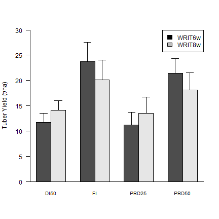
Figure 1
Average ± standard error (n = 4) of tuber yield in four irrigation treatments at two irrigation onset timing: 6 (WRIT6w) and 8 (WRIT8w) weeks after planting. Different letters indicate differences (P < 0.05).
For WRIT6w group
# average yield for each irrigation treatment
yield6_TRT <- tapply(ty_WRIT6W$TY, ty_WRIT6W$TRT, mean)
# standard deviation
yield6_TRT_sd <- tapply(ty_WRIT6W$TY, ty_WRIT6W$TRT, sd)
# number of observation per irrigation treatment
yield6_TRT_n <- tapply(ty_WRIT6W$TY, ty_WRIT6W$TRT, length)
# standard error
yield6_TRT_sem <- yield6_TRT_sd / sqrt(yield6_TRT_n)
for the WRIT8w group
# Mean
yield8_TRT <- tapply(ty_WRIT8W$TY,ty_WRIT8W$TRT, mean)
# Standard error
yield8_TRT_sem <- tapply(ty_WRIT8W$TY,ty_WRIT8W$TRT,sd)/sqrt(tapply(ty_WRIT8W$TY,ty_WRIT8W$TRT, length))
Combine mean yield and standard error to make a plot
yield_TRT <- cbind(WRIT6w=yield6_TRT, WRIT8w=yield8_TRT)
yield_TRT_sem <- cbind(yield6_TRT_sem, yield8_TRT_sem)
Make a barplot
mids <- barplot(t(yield_TRT), beside=T, ylab="Tuber Yield (t/ha)",
          cex.names=0.8, las=1, ylim=c(0,30))
# Add the bottom line
box(bty="l")
# Add legend
legend("topright", fill = c("black", "grey"), c("WRIT6w", "WRIT8w"), horiz = F)
# Add standard erros to the plot (only the postive part)
arrows (mids, t(yield_TRT), mids, t(yield_TRT + yield_TRT_sem), code = 3, angle = 90, length = .1)
Check significance to plot, HSD.test and TukeyHSD both can be used.
library(agricolae)
## Warning: package 'agricolae' was built under R version 4.3.1
yield6TRT_aov <- aov(ty_WRIT6W$TY ~ ty_WRIT6W$TRT)
a <- HSD.test(yield6TRT_aov, trt = "ty_WRIT6W$TRT" )
yield8TRT_aov <- aov(ty_WRIT8W$TY ~ ty_WRIT8W$TRT)
# Method 1
b <- TukeyHSD(yield8TRT_aov)
# Method 2
b1 <- HSD.test(yield8TRT_aov, trt = "ty_WRIT8W$TRT" )
### plot values are similar but not the siginificance.
Table 3
F-values of ANOVA with repeated measurements in time corresponding to leaflet relative water content (RWC) obtained at two water restriction initiation timing: 6 (WRIT6w) and 8 (WRIT8w) weeks after planting. Take WRIT8w goup as an example.
# In the table, there are observations for different time, need to reorgnize the data, to make time as a factor
rwc = reshape(rwc8[,-1], varying = c("10DAT", "28DAT", "39DAT", "52DAT"), idvar=c("B", "TRT"), direction="long", v.names="RWC", times=c(10, 28, 39, 52))
rwc$time <- as.factor(rwc$time)
Build a liner regression model and do ANOVA
model <- lm(RWC ~ block + TRT + time + TRT*time, data = rwc)
## Error in eval(predvars, data, env): object 'block' not found
anova(model)
## Error in eval(expr, envir, enclos): object 'model' not found
Similar resutls but not the same values.
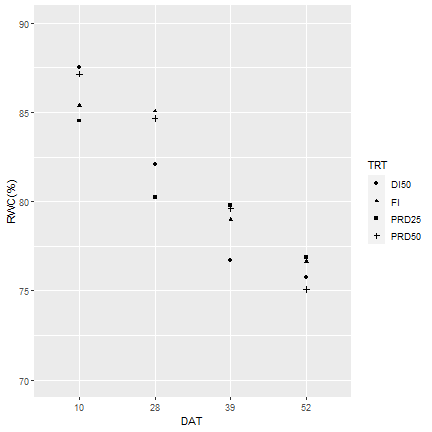
3.5. figure 2
Average ± standard error of relative water content (RWC) under four irrigation treatments at water restriction initiation timing 6 (WRIT6w) weeks after planting was shown as an exmple. ** P < 0.01, *P < 0.05, n.s. = no significant (P > 0.05). DAT = days after treatment.
Effect irigation treatment on RWC for each date
times <- c(10, 28, 39, 52)
lapply(times, function(i) anova(lm(RWC ~ TRT, data=rwc[rwc$time==i, ])))
## [[1]]
## Analysis of Variance Table
##
## Response: RWC
##           Df  Sum Sq Mean Sq F value Pr(>F)
## TRT        3  24.676  8.2254  0.4794 0.7026
## Residuals 12 205.911 17.1593
##
## [[2]]
## Analysis of Variance Table
##
## Response: RWC
##           Df Sum Sq Mean Sq F value Pr(>F)
## TRT        3  62.85  20.952  0.6287 0.6103
## Residuals 12 399.90  33.325
##
## [[3]]
## Analysis of Variance Table
##
## Response: RWC
##           Df  Sum Sq Mean Sq F value Pr(>F)
## TRT        3  24.126  8.0419  0.4042 0.7527
## Residuals 12 238.763 19.8969
##
## [[4]]
## Analysis of Variance Table
##
## Response: RWC
##           Df  Sum Sq Mean Sq F value Pr(>F)
## TRT        3   8.255  2.7516  0.1776 0.9095
## Residuals 12 185.886 15.4905
f <- function(i) {
  d <- rwc[rwc$time==i, ]
  anov <- aov(RWC ~ TRT, data=d)
  HSD.test(anov, trt = "TRT")$groups
}
lapply(times, f)
## [[1]]
##            RWC groups
## DI50  87.53202      a
## PRD50 87.15764      a
## FI    85.37740      a
## PRD25 84.52310      a
##
## [[2]]
##            RWC groups
## FI    85.07299      a
## PRD50 84.65415      a
## DI50  82.05848      a
## PRD25 80.20828      a
##
## [[3]]
##            RWC groups
## PRD25 79.76402      a
## PRD50 79.60296      a
## FI    78.97143      a
## DI50  76.69406      a
##
## [[4]]
##            RWC groups
## PRD25 76.87319      a
## FI    76.62935      a
## DI50  75.76053      a
## PRD50 75.06475      a
No siginificance difference among irrigation treatments for each date
Use aggregate to caculate mean RWC for different time and irrigation treatement
rwc_agg <- aggregate(rwc[, 'RWC', drop=FALSE], rwc[, c('time',"TRT")], function(i) cbind(mean(i), sd(i), length(i)))
rwc_agg <- cbind(rwc_agg[,-3], rwc_agg[,3])
colnames(rwc_agg)[3:5] <- c("mean", "sd", "n")
dim(rwc_agg)
## [1] 16  5
# Standard error
rwc_agg$sem <- rwc_agg$sd / sqrt(rwc_agg$n)
# Make a qqplot this time
library(ggplot2)
qplot(data = rwc_agg, x = as.factor(time), y = mean, pch= TRT, xlab = "DAT", ylab = "RWC(%)", ylim = c(70,90))
## Warning: `qplot()` was deprecated in ggplot2 3.4.0.
## This warning is displayed once every 8 hours.
## Call `lifecycle::last_lifecycle_warnings()` to see where this warning was generated.
#+ geom_errorbar(aes(ymin = rwc_agg$mean - rwc_agg$sem, ymax = rwc_agg$sem + rwc_agg$mean), colour="black", width=.05)