Sweetpotato Cultivar Selection
Introduction
This case study looks at data from a study on sweetpotato cultivars in Mozambique. Specifically, we will demonstrate methodology used in the article published in Genotype x Environment interaction and selection for drought adaptation in sweetpotato in Mozambique. In this study, 58 cultivars were evaluated over three years, looking at performance under both full irrigation and limited irrigation. Methods used include analysis of variance, regression, and additive main effects multiplicative interaction (AMMI), which will be shown in this case study.
The data used is available on the CIP datavarse. Unfortunately, the dataset is missing data from the 2009 study, so we will use the same methodology with only 2006 and 2008 data. Results will differ from those reported in the paper.
Download
library(agro)
ff <- get_data_from_uri("https://data.cipotato.org/dataset.xhtml?persistentId=doi:10.21223/P3/M0HGJ4", ".")
ff
## [1] "./doi_10.21223_P3_M0HGJ4/Cluster_Analysis_Drought.xlsx"
## [2] "./doi_10.21223_P3_M0HGJ4/Data_Dictionary_Drought.xlsx"
## [3] "./doi_10.21223_P3_M0HGJ4/Drought_06_08.xls"
Read
The dataset consisits of three files, including the data itself,
information on the clones, and a data dictionary. Two of the files are
“.tab”, and the third is an excel file. Below, we read in each of the
files in the dataset. To read the excel file we use the readxl
package.
Now that we have the files, we can read them into R.
cluster <- read.delim(ff[1], stringsAsFactors=FALSE)
## Warning in read.table(file = file, header = header, sep = sep, quote = quote, :
## line 1 appears to contain embedded nulls
## Warning in read.table(file = file, header = header, sep = sep, quote = quote, :
## incomplete final line found by readTableHeader on
## './doi_10.21223_P3_M0HGJ4/Cluster_Analysis_Drought.xlsx'
## Error in type.convert.default(data[[i]], as.is = as.is[i], dec = dec, : invalid multibyte string at '<ef><ef><d3>'
dict <- read.delim(ff[2], stringsAsFactors=FALSE)
## Warning in read.table(file = file, header = header, sep = sep, quote = quote, :
## line 1 appears to contain embedded nulls
## Warning in read.table(file = file, header = header, sep = sep, quote = quote, :
## line 5 appears to contain embedded nulls
## Warning in read.table(file = file, header = header, sep = sep, quote = quote, :
## incomplete final line found by readTableHeader on
## './doi_10.21223_P3_M0HGJ4/Data_Dictionary_Drought.xlsx'
## Error in read.table(file = file, header = header, sep = sep, quote = quote, : more columns than column names
library(readxl)
drought <- read_excel(ff[3])
We need to convert some our variables of interest to numeric. The reason
is that some records for these variable have the odd values “*”. I first
set these to NA to avoid the warning NAs introduced by coercion.
You need to treat warnings like errors, never ignore them, and make them
go away if you can.
drought$RYTHA[drought$RYTHA == "*"] <- NA
drought$FYTHA[drought$FYTHA == "*"] <- NA
drought$BIOM[drought$BIOM == "*"] <- NA
Now the conversion
drought$RYTHA <- as.numeric(drought$RYTHA)
drought$FYTHA <- as.numeric(drought$FYTHA)
drought$BIOM  <- as.numeric(drought$BIOM)
Remove NAs
drought <- drought[!is.na(drought$RYTHA),]
Summary Statistics
First, we will plot some graphs to demonstrate basic summary statistics of the data. We will use the package ‘ggplot’, which has more flexibility in the plots produced. We begin by adding an important variable to the data, environment (a combination of year and treatment), then plot a histogram and boxplot.
To create a variable environment we combine the year and treatment
(irrigated/non-irrigated)
drought$env <- as.factor(paste(drought$YEAR, drought$TREATMENT))
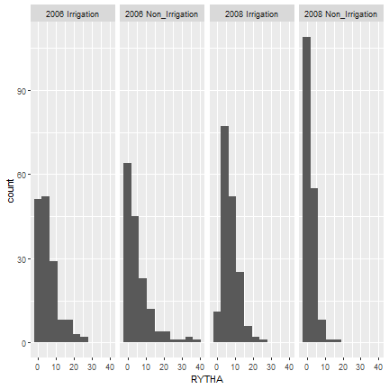
First, we will represent the data with a histogram, using the argument ‘geom_histogram’. This shows us the differences in distribution of observations in the four environments of interest. We can see that in both non-irrigated environments, the majority of observations fall in the smallest bin, while this is not the case for the irrigated environments.
library(ggplot2)
ggplot(drought, aes(x=RYTHA)) +
  geom_histogram(bins=10) +
  facet_wrap(~drought$env, nrow=1)
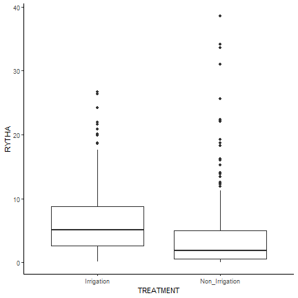
Next, we can represent the data with a box plot. Here we graph the distribution of the two treatments, irrigated and non-irrigated. From initial observation, it appears that the irrigated plots had higher and less variable root yields than the non-irrigated plots.
ggplot(drought, aes(y=RYTHA, x=TREATMENT, fill = REP)) +
  geom_boxplot() +
  theme_classic()
## Warning: The following aesthetics were dropped during statistical transformation: fill
## ℹ This can happen when ggplot fails to infer the correct grouping structure in the data.
## ℹ Did you forget to specify a `group` aesthetic or to convert a numerical variable into a factor?
The article makes a distinction between farmer landraces and bred/modern cultivars. In the dataframe “cluster”, we can split the cultivars between farmer landraces and modern varieties, following the distinction on table 5 of the paper. Here we show boxplots for four variables of interest: dry matter (DM), total biomass (BIOM), harvest index (HI), and geometric mean (GM). For more information on these variables, see the table ‘dict’. We also use the package ‘gridExtra’ to plot all the graphs at once.
#New variable for type of cultivar
cluster$type <- as.numeric(row.names(cluster))
## Error in eval(expr, envir, enclos): object 'cluster' not found
#The first 40 cultivars are landrace, the rest are modern (refer to table 5)
cluster$type <- ifelse(cluster$type <41, "landrace", "modern")
## Error in eval(expr, envir, enclos): object 'cluster' not found
#Remove x-asis title (on first two) and legend (on all) to avoid repetition
p1 <- ggplot(cluster, aes(y=DM, x=type, color=type)) +
  geom_boxplot()+
  theme(legend.position="none", axis.title.x=element_blank())
## Error in eval(expr, envir, enclos): object 'cluster' not found
p2 <- ggplot(cluster, aes(y=BIOM, x=type, color=type)) +
  geom_boxplot()+
  theme(legend.position="none", axis.title.x=element_blank())
## Error in eval(expr, envir, enclos): object 'cluster' not found
p3 <- ggplot(cluster, aes(y=HI, x=type, color=type)) +
  geom_boxplot()+
  theme(legend.position="none")
## Error in eval(expr, envir, enclos): object 'cluster' not found
p4 <- ggplot(cluster, aes(y=GM, x=type, color=type)) +
  geom_boxplot()+
  theme(legend.position="none")
## Error in eval(expr, envir, enclos): object 'cluster' not found
g_legend <- function(a.gplot) {
  tpm <- ggplot_gtable(ggpl)
}
library(gridExtra)
grid.arrange(p1, p2, p3, p4, nrow=2)
## Error in eval(expr, envir, enclos): object 'p1' not found
Cluster Analysis
The authors use cluser analysis to show linkages between the different cultivars, based on many of the variables of interest: geometric yield, drought sensitivity index, drought tolerance expression, percent reduction, harvest index, and root dry matter. Below, we do the same using the function ‘hclust’.
row.names(cluster) <- cluster$Cultivar
## Error in eval(expr, envir, enclos): object 'cluster' not found
j <- hclust(dist(cluster[,c(2,3,5,7,8)]), method="average")
## Error in eval(expr, envir, enclos): object 'cluster' not found
plot(j, xlab="Cultivar", hang= -1, cex = 0.6)
## Error in eval(expr, envir, enclos): object 'j' not found
Analysis of Variance
The performance of cultivars was assessed with analysis of variance. The three traits of interest were storage root yield, vine yield, and biomass, and were observed across variation in environment (E), genotype (G), and G x E. While the study reports 5 degrees of freedom for the environment, we will only have 3 since we are missing data from 2009. We will report the mean square, stability variance, and relative variance as shown in Table 3 of the paper. In this section, we will use the function ‘aov’ for analysis of variance.
#Storage Root Yield
RYTHA.anova <- aov(RYTHA ~ env + CULTIVAR + CULTIVAR*env, data=drought)
summary(RYTHA.anova)
##               Df Sum Sq Mean Sq F value Pr(>F)
## env            3   2200   733.2  69.486 <2e-16 ***
## CULTIVAR      57   6784   119.0  11.280 <2e-16 ***
## env:CULTIVAR 170   5048    29.7   2.814 <2e-16 ***
## Residuals    427   4506    10.6
## ---
## Signif. codes:  0 '***' 0.001 '**' 0.01 '*' 0.05 '.' 0.1 ' ' 1
#Vine Yield
FYTHA.anova <- aov(FYTHA ~ env + CULTIVAR + CULTIVAR*env, data=drought)
summary(FYTHA.anova)
##               Df Sum Sq Mean Sq F value   Pr(>F)
## env            3  27944    9315  90.332  < 2e-16 ***
## CULTIVAR      57  68062    1194  11.580  < 2e-16 ***
## env:CULTIVAR 170  31036     183   1.771 1.86e-06 ***
## Residuals    425  43824     103
## ---
## Signif. codes:  0 '***' 0.001 '**' 0.01 '*' 0.05 '.' 0.1 ' ' 1
## 2 observations deleted due to missingness
#Biomass
BIOM.anova <- aov(BIOM ~ env + CULTIVAR + CULTIVAR*env, data=drought)
summary(BIOM.anova)
##               Df Sum Sq Mean Sq F value   Pr(>F)
## env            3  43828   14609  113.66  < 2e-16 ***
## CULTIVAR      57  76124    1336   10.39  < 2e-16 ***
## env:CULTIVAR 170  40432     238    1.85 2.98e-07 ***
## Residuals    425  54630     129
## ---
## Signif. codes:  0 '***' 0.001 '**' 0.01 '*' 0.05 '.' 0.1 ' ' 1
## 2 observations deleted due to missingness
Regression
Next, we replicate table 4, which uses linear regression and takes into account interactions between environment and genotypes.
#create dummy variables for the different environments
drought$IR6 <- ifelse(drought$env=="2006 Irrigation", 1, 0)
drought$NI6 <- ifelse(drought$env=="2006 Non_Irrigation", 1, 0)
drought$IR8 <- ifelse(drought$env=="2008 Irrigation", 1, 0)
drought$NI8 <- ifelse(drought$env=="2008 Non_Irrigation", 1, 0)
#To see the effect of each environment on root yield, we can use the linear model with root yield as the y axis, and each environment as the x-axis.
linear <- lm(RYTHA ~IR6 + NI6 + IR8, data=drought)
summary(linear)
##
## Call:
## lm(formula = RYTHA ~ IR6 + NI6 + IR8, data = drought)
##
## Residuals:
##    Min     1Q Median     3Q    Max
## -6.938 -3.341 -1.464  1.994 32.868
##
## Coefficients:
##             Estimate Std. Error t value Pr(>|t|)
## (Intercept)   2.2562     0.3789   5.955 4.26e-09 ***
## IR6           3.2641     0.5539   5.893 6.09e-09 ***
## NI6           3.4561     0.5502   6.282 6.10e-10 ***
## IR8           4.8595     0.5359   9.069  < 2e-16 ***
## ---
## Signif. codes:  0 '***' 0.001 '**' 0.01 '*' 0.05 '.' 0.1 ' ' 1
##
## Residual standard error: 4.998 on 654 degrees of freedom
## Multiple R-squared:  0.1187, Adjusted R-squared:  0.1146
## F-statistic: 29.35 on 3 and 654 DF,  p-value: < 2.2e-16
#Because we have so many cultivars, we can make them into dummy variables with the following code:
cultivar.f = factor(drought$CULTIVAR)
dummies = model.matrix(~cultivar.f)
linear2 <- lm(drought$RYTHA ~ dummies)
#summary(linear2)
AMMI Model
The fourth step used in this article for the analysis of sweet potato
cultivars is the additive main effects and multiplicative interactions
model (AMMI). AMMI combines both ANOVA methodology (additive) and PCA
(multiplicative) to better understand how environments and genotypes
interact. Here, we will use the AMMI function from the agricolae
package.
library(agricolae)
## Warning: package 'agricolae' was built under R version 4.3.1
#To make for easier viewing, we will use the codes rather than cultivar names, as charactes.
drought$CODE_CULTIVAR <- as.character(drought$CODE_CULTIVAR)
#the function AMMI specifies the environment variable, genotype, and repition, as well as the y-variable of interest.
ammi <- AMMI(ENV=drought$env, GEN=drought$CODE_CULTIVAR, REP=drought$REP, Y = drought$RYTHA, PC=T)
ammi$ANOVA
## Analysis of Variance Table
##
## Response: Y
##            Df Sum Sq Mean Sq F value    Pr(>F)
## ENV         3 2199.6  733.20 15.9863 0.0009673 ***
## REP(ENV)    8  366.9   45.86  4.6448 1.867e-05 ***
## GEN        57 6770.1  118.77 12.0284 < 2.2e-16 ***
## ENV:GEN   170 5063.1   29.78  3.0162 < 2.2e-16 ***
## Residuals 419 4137.4    9.87
## ---
## Signif. codes:  0 '***' 0.001 '**' 0.01 '*' 0.05 '.' 0.1 ' ' 1
ammi$analysis
##     percent  acum Df    Sum.Sq   Mean.Sq F.value Pr.F
## PC1    58.9  58.9 59 3171.8441 53.760070    5.44    0
## PC2    37.2  96.1 57 2005.9770 35.192580    3.56    0
## PC3     3.9 100.0 55  207.6749  3.775907    0.38    1
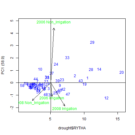
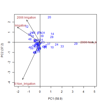
We can graph the results from the ammi model on a bi-plot. Below we plot two biplots. The first shows the first and second principal componenets plotted against each other, and the second shows the first principal component plotted against the yield variable.
#The regular plot(ammi) will plot PC1 against PC2
plot(ammi)
#To graph the dependent variable against pc1, the following code is used. 0 is the y-dependent variable (RYTHA), and 1 is PC1.
plot(ammi, 0, 1, gcol="blue", ecol="green")