MODIS data pre-processing¶

In this chapter we download, pre-process and compute NDVI from MODIS data. These procedures are discussed in more detail here.

Area of interest¶

First we get the area of interest. Normally you would get this from a file (for example, a shapefile). See ?terra::vect for reading such files.

aoi <- agrodata::data_ibli("marsabit")
aoi
##  class       : SpatVector
##  geometry    : polygons
##  dimensions  : 58, 8  (geometries, attributes)
##  extent      : 36.18001, 38.96632, 1.261462, 4.452989  (xmin, xmax, ymin, ymax)
##  coord. ref. : +proj=longlat +datum=WGS84 +no_defs
##  names       : COUNTRY PROVINCE DISTRICT     DIVISION      LOCATION
##  type        :   <chr>    <chr>    <chr>        <chr>         <chr>
##  values      :   KENYA  EASTERN MARSABIT LOIYANGALANI      MT KULAL
##                  KENYA  EASTERN MARSABIT     GADAMOJI        BADASA
##                  KENYA  EASTERN MARSABIT   NORTH HORR BALESA RIRIBA
##  SUB_LOCATION IBLI_UNIT IBLI_ID
##         <chr>     <chr>   <num>
##        ARAPAL  MT KULAL     115
##        BADASA  GADAMOJI     112
##        BALESA    DUKANA     119

As you can see we have 58 polygons, each representing a “sub-location”. Let’s plot the polygons on top of a map of Kenya to see where they are.

library(terra)
ken <- geodata::gadm("KEN", level=1, path=".")
plot(ken, border="gray")
plot(ken[ken$NAME_1 == "Marsabit", ], col="beige", border="gray", add=TRUE)
lines(aoi, col="red")

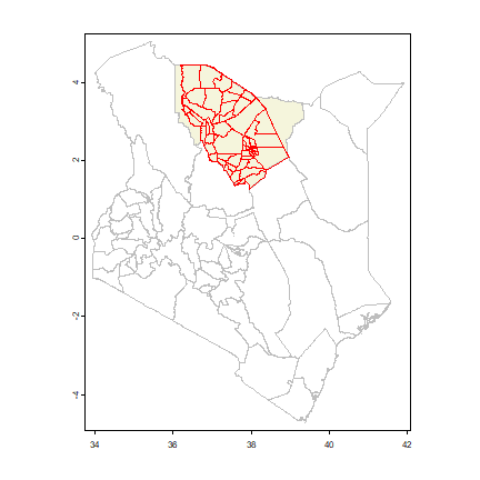
So we are in Northe Kenya. Also note that some polygons (sub-locations) are much smaller than others.

Get MODIS files¶

Here we show how to download and pre-process the data, but only for 1 month, to limit the download and processing needed. After that we use pre-processed data.

Set up the download directory

datadir <- "modis"
dir.create(datadir, FALSE)
# datadir

In this example we download data from 2010 only.

start <- "2010-01-01"
end <- "2010-01-07"

To download the data you need to provide the username and password for your (free) EOSDIS account. If you do not have an account, you can sign up here. Here we use passwords that are stored in a file that I read in below (sorry, we cannot show you the values).

up <- readRDS("../pwds.rds")
up <- up[up$service == "EOSDIS", ]

Now we are ready to get the data

library(luna)
fmod <- luna::getModis(product="MOD09A1", start, end, aoi, download=TRUE,
            path=datadir, username=up$user, password=up$pwd)
fmod
## [1] "modis/MOD09A1.A2009361.h21v08.061.2021149144347.hdf"
## [2] "modis/MOD09A1.A2010001.h21v08.061.2021150093948.hdf"
## [3] "modis/MOD09A1.A2009361.h21v08.006.2015198070255.hdf"
## [4] "modis/MOD09A1.A2010001.h21v08.006.2015198080805.hdf"

We only have four files here, each representing 8 days – just to illustrate the processing.

A single MODIS tile for extends well over the study area. We first crop the data to correspond to the study area, and then we remove bad pixels (clouds and shadow) and then .

Quality¶

To remove bad quality pixels from the selected files, we follow the same method described here. We specify a matrix in which each row has start and end of the quality assessment (QA) bits considered, and the values to be rejected (in the image).

from <- c(1,3,11,12)
to   <- c(2,6,11,14)
reject <- c("10,11", "1100,1101,1110,1111", "1", "000,110,111")
qmat <- cbind(from, to, reject)

We need to project the case study boundary to the sinusoidal coordinate reference system that the MODIS data are in.

prj <- "+proj=sinu +lon_0=0 +x_0=0 +y_0=0 +a=6371007.181 +b=6371007.181 +units=m +no_defs "
pols <- project(aoi, prj)

Monthly NDVI computation¶

We now compute NDVI for each month. First, produce a quality mask, mask out bad quality pixels, crop to the area of interest, and then compute NDVI.

We use a loop over all files (fmod).

for(i in seq_along(fmod)) {
  # Load a MODIS file
  r <- rast(fmod[i])
  # Generate quality mask (layer 12)
  quality_mask <- modis_mask(r[[12]], 16, qmat)
  #Select only red and NIR
  r <- r[[1:2]]
  names(r) <- c("red", "NIR")
  # remove low quality pixels
  r <- mask(r, quality_mask)
  # remove areas outside the AOI rectangle
  r <- crop(r, pols)
  # ensure that all values are between 0 and 1
  r <- clamp(r, 0, 1)
  # Compute NDVI
  ndvi <- (r$NIR - r$red)/(r$NIR + r$red)
  filename <- gsub(".hdf$", "_ndvi.tif", fmod[i])
  writeRaster(ndvi, filename=filename, overwrite=TRUE)
}