Livestock mortality
Introduction
In this section we explore Marsabit household survey data collected by ILRI in Marsabit between 2008 and 2015.
First let us explore losses table dataset.
d <- agrodata::data_ibli("marsabit_losses")
d[1:5, c(1:6, 9:10)]
##     hhid sublocation year month     animal              cause totalloss
## 342 1002 DAKABARICHA 2009     7     Cattle Starvation/Drought         2
## 343 1002 DAKABARICHA 2009     8 Goat/Sheep Starvation/Drought         3
## 344 1002 DAKABARICHA 2009     9     Cattle Starvation/Drought         2
## 345 1002 DAKABARICHA 2011     6     Cattle Starvation/Drought         1
## 346 1002 DAKABARICHA 2011     8     Cattle Starvation/Drought         3
##     adultloss
## 342         1
## 343         3
## 344         2
## 345         1
## 346         1
Here is a list of the variables we have access to.
name |
description |
|---|---|
hhid |
unique household ID |
sublo catio n |
sublocation name |
year |
year of loss event |
month |
month of loss event |
anima l |
animal species |
cause |
cause of loss |
cause _othe r |
other causes not on list |
where |
at base or satellite camp? |
total loss |
number of animals lost? |
adult loss |
number of adult animals lost (>= 3 years for cattle/camel, >= 6 months for sheep/goat) |
From the data we can observer three livestock species.
table(d$animal)
##
##      Camel     Cattle Goat/Sheep
##       2173       2231       8177
x <- tapply(d$totalloss, d$animal, sum, na.rm=TRUE)
barplot(x, col=rainbow(3), las=1)
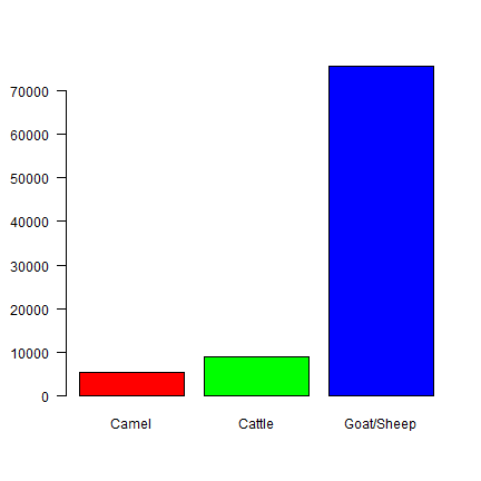
There are many more “shoats” (sheep/goats) that die. But 1 cow is much more valuable than 1 goat. One way to compare these species better, is to use Tropical Livestock Units (TLUs). A cow has a value of 1, camel 1.429 (1/0.7), and a shoat has a TLU value of 0.1 (1/10). Compute TLU values for each animal type.
x
##      Camel     Cattle Goat/Sheep
##       5340       8839      75674
tlu <- c(camel=1.4, cattle=1, shoat=0.1)
xtlu <- x * tlu
barplot(xtlu, col=rainbow(3), las=1)
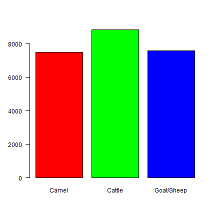
In terms of TLU, overall mortality is about the same for each species. We can also use TLU to combine the species.
animals <- match(trimws(d$animal), c("Goat/Sheep", "Camel", "Cattle"))
anitlu <- tlu[animals]
youngloss <- d$totalloss - d$adultloss
d$tluloss <- (d$adultloss + youngloss/2) * anitlu
Now we can sum up the number of TLUs lost per month.
a <- aggregate(d[, "tluloss", drop=FALSE], d[, c("year", "month")], sum, na.rm=TRUE)
a <- a[order(a$year, a$month), ]
time <- as.Date(paste(a$year, a$month, 15, sep="-"))
plot(time, a$tluloss, ylab="Loss (TLU)")
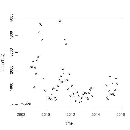
We see high overall losses in 2009 and 2011. In the next chapter we will relate these losses to NDVI.
The losses in 2008 are very low (because data collection started in 2009). Also note that no household survey was done in 2014 as noted in code book.
xtabs(tluloss ~ month+year, d)
##      year
## month    2008    2009    2010    2011    2012    2013    2014    2015
##    1    14.00 1003.35  295.45 1436.90 1079.35  648.00    0.00  793.60
##    2    11.20 2124.40  347.15 4816.50 1055.65  679.20    0.00 1617.05
##    3     2.10 1766.80  414.35 1625.10  610.50  635.80    0.00  595.70
##    4     1.40 2552.85  390.45 1298.80  417.80  404.35    0.00 1221.45
##    5     5.70 2743.20  335.15 2035.70  202.00  319.95    0.00  611.10
##    6    13.30 4164.45  546.85 1780.80  751.85  655.25    0.00  546.55
##    7    56.35 4655.80  900.45 3757.85  732.25  855.50    0.00  834.30
##    8     2.45 4606.30  941.65 3489.00  492.75  958.30    0.00 1504.40
##    9    31.80 3717.05  394.70 1423.60  157.40  504.85    0.00 1190.50
##    10 2148.30 1553.60  285.55  878.80  177.95    0.00 1120.65    0.00
##    11 2179.25  845.85  821.75 1778.35  390.55    0.00  447.60    0.00
##    12 2477.55  795.60 1063.65  496.45  591.85    0.00  317.60    0.00
Causes of death
cause <- tapply(d$tluloss, d$cause, sum, na.rm=TRUE)
x <- sort(round(cause))
par(mai=c(1,2,1,1))
barplot(x, horiz=T, las=1)
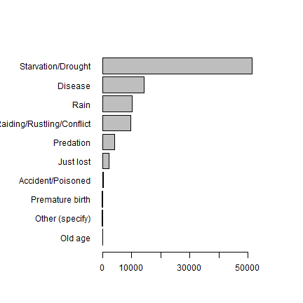
Clearly starvation associated with drought is a major cause of death, followed by disease.
Let’s simplify to three classes.
i <- d$cause %in% c("Starvation/Drought", "Disease")
d$cause2 <- "Other"
d$cause2[i] <- d$cause[i]
d$cause2[d$cause2 == "Starvation/Drought"] <- "Starvation"
And now we aggregate the values by calendar year.
yc <- aggregate(d[, "tluloss", drop=FALSE], d[, c("cause2", "year")], sum, na.rm=TRUE)
head(yc)
##       cause2 year  tluloss
## 1    Disease 2008  1122.75
## 2      Other 2008  3654.35
## 3 Starvation 2008  2941.00
## 4    Disease 2009  2649.95
## 5      Other 2009  4330.40
## 6 Starvation 2009 23548.90
Some more manipulation to create a stacked barplot.
r <- reshape(yc, direction="wide", idvar="cause2", timevar="year")
colnames(r) <- gsub("tluloss.", "", colnames(r))
r <- as.matrix(r)
rownames(r) <- r[,1]
barplot(r[,-1], legend =  rownames(r), las=2, args.leg=list(cex=1))
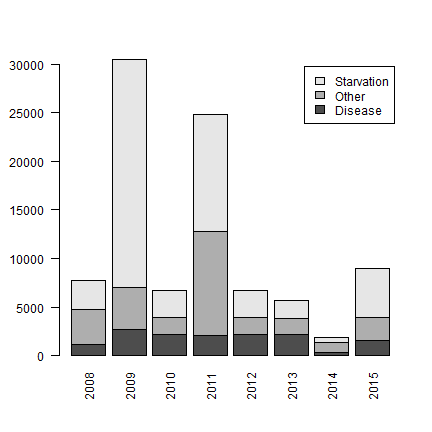
Again we see two outlier years with very high losses. In the other years, we also see some starvation, but generally there are more losses because of disease and other factors.