Modeling mortality
Introduction
To design and evaluate an index based insurance contract, we need to understand the relationship between the index and losses incurred. Here we develop such a relationship using the z-scored NDVI to predict livestock mortality, using survey data from Marsabit.
Data
Mortality
Mortality was computed from survey data collected in Marsabit between 2008 and 2015. First read the data.
mort <- agrodata::data_ibli("marsabit_mortality.rds")
mort[1:5, 1:7]
##   hhid season year sublocation           type     stock loss
## 1 1002   SRSD 2008 DAKABARICHA          Camel  0.000000    0
## 2 1002   SRSD 2008 DAKABARICHA         Cattle 13.000000    0
## 3 1002   SRSD 2008 DAKABARICHA          Shoat  4.000000    0
## 4 1002   SRSD 2008 DAKABARICHA            TLU 13.400000    0
## 5 1002   SRSD 2008 DAKABARICHA TLU per capita  1.914286    0
Load data with causes of death.
cause <- agrodata::data_ibli("marsabit_losses")
cause <- cause[,c("hhid", "sublocation", "cause","month", "year")]
colnames(cause)[4] <- "season"
s <- cause$season
cause$season <- "SRSD"
cause$season[s >=3 & s <=9] <-"LRLD"
cause <- na.omit(cause)
head(cause, n=2)
##     hhid sublocation              cause season year
## 342 1002 DAKABARICHA Starvation/Drought   LRLD 2009
## 343 1002 DAKABARICHA Starvation/Drought   LRLD 2009
Merge this table with mortality table and extract mortality causes by starvation/drought.
mort <- merge(mort, cause, by=c("hhid","sublocation", "season", "year"))
mort <- mort[mort$cause == "Starvation/Drought", ]
We mainly care about the mortality rates. Compute aggregates by year, season and sublocation.
mort <- mort[mort$type == "TLU", ]
amort <- aggregate(mort[,c("stock_beginning", "loss")], mort[ , c("year", "season", "sublocation")], sum, na.rm=TRUE)
head(amort, n=2)
##   year season sublocation stock_beginning   loss
## 1 2009   LRLD      BUBISA          8936.4 2072.0
## 2 2010   LRLD      BUBISA           520.3   40.4
amort$mortality_rate = 1 - ((amort$stock_beginning - amort$loss) / amort$stock_beginning )
amort$mortality_rate[amort$mortality_rate==0] <- NA
NDVI
Load the zNDVI data for 2000–2015 and income data for Marsabit that we computed in the previous section. We reshape the data from “wide” to “long” format.
LR <- agrodata::data_ibli("marsabit_zLRLD")
SR <- agrodata::data_ibli("marsabit_zSRSD")
LR[1:3, 1:6]
##   sublocation   LRLD2000  LRLD2001   LRLD2002  LRLD2003   LRLD2004
## 1      ARAPAL -2.0961337 0.3242631 -0.3526237 1.1115084  0.3370314
## 2      BADASA -0.6657791 0.2393530  0.6495006 0.9258476  0.6766376
## 3      BALESA -1.0856171 0.1699284 -0.2237794 1.4356138 -0.3569806
lr <- reshape(LR, direction="long", varying = 2:ncol(LR), v.names="NDVI", timevar="year", times=2000:2015)
lr$id <- "LRLD"
sr <- reshape(SR, direction="long", varying = 2:ncol(LR), v.names="NDVI", timevar="year", times=2000:2015)
sr$id <- "SRSD"
ndvi <- rbind(lr, sr)
colnames(ndvi)[4] <- "season"
ndvi$year_season <- apply(ndvi[, c("year", "season")], 1, function(x) paste(x, collapse="_"))
head(ndvi, n=2)
##        sublocation year       NDVI season year_season
## 1.2000      ARAPAL 2000 -2.0961337   LRLD   2000_LRLD
## 2.2000      BADASA 2000 -0.6657791   LRLD   2000_LRLD
Merge mortality and NDVI
d <- merge(ndvi, amort, by=c("year", "season", "sublocation"))
Explore the relation between mortality and NDVI.
cols <- c("red", "blue")
seas <- c("SRSD", "LRLD")
pcols <- cols[match(d$season, seas)]
plot(mortality_rate~NDVI, data=d, xlab="zndvi", ylab="mortality", col=pcols, pch=20)
legend("topright", seas, col=cols, pch=20)
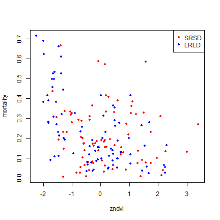
The relationship is a bit noisy (as to be expected). There is a lot of variability at zNDVI < -1. That could be a problem; as predictions of mortality at low zNDVI would be quite uncertain.
Mortality model
Build a local regression model.
dd <- na.omit(d[, c("NDVI", "mortality_rate")])
# add two "anchering points"
dd <- rbind(dd, c(-2.5, 0.9))
dd <- rbind(dd, c(-4, 1))
saveRDS(dd, "ndvi_mort.rds")
library(msir)
## Warning: package 'msir' was built under R version 4.3.1
## Package 'msir' version 1.3.3
## Type 'citation("msir")' for citing this R package in publications.
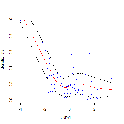
# Calculate and plot a 1.96 * SD prediction band
# that is a 95% prediction band
m <- loess.sd(dd)
plot(dd, cex=.5, col="blue", xlab="zNDVI", ylab="Mortality rate")
lines(m$x, m$y, col="red")
lines(m$x, m$upper, lty=2)
lines(m$x, m$lower, lty=2)
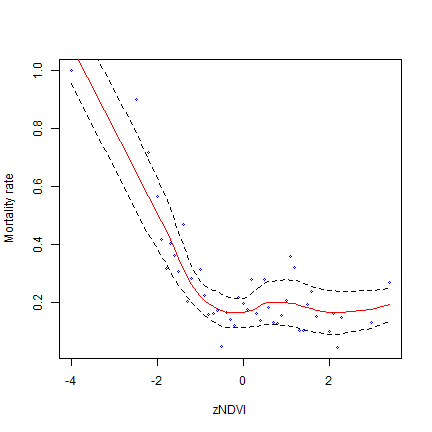
Same thing after a little generalization.
x <- dd
x$NDVI = round(x$NDVI, 1)
a <- aggregate(x[, "mortality_rate", drop=FALSE], x[, "NDVI", drop=FALSE], mean)
ma <- loess.sd(a)
plot(a, cex=.5, col="blue", xlab="zNDVI", ylab="Mortality rate")
lines(ma$x, ma$y, col="red")
lines(ma$x, ma$upper, lty=2)
lines(ma$x, ma$lower, lty=2)
Compare predicted with observed mortality rates
ml <- loess(mortality_rate ~ NDVI, data=dd)
p <- predict(ml, d)
plot(d$mortality_rate, p, xlab="mortality rate", ylab="predicted")
abline(0,1)
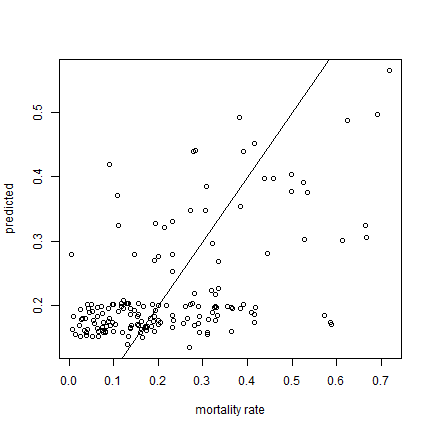
x <- na.omit(cbind(d$mortality_rate, p))
cor(x[,1], x[,2])
## [1] 0.5567935
d$predicted_mortality <- p
saveRDS(d, "pred_mort1.rds")
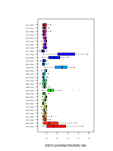
Predict mortality in other years based on their zNDVI.
ndvi$predicted_mortality <- predict(ml, ndvi)
par(mai=c(1,2,1,1))
boxplot(ndvi$predicted_mortality ~ ndvi$year_season, las=1, cex.axis=.5, horizontal=TRUE, xlab="zNDVI predicted Mortality rate", ylab="", cex=.25, col=rainbow(32))
saveRDS(ndvi, "pred_mort2.rds")