Mapping rice area
Introduction
Different methods for crop mapping have been developed using remote sensing data. The most common approach is supervised classification, and we worked through an example of that in week 2.
Here we use a different, rule-based, approach that uses time-series of remote-sensing data to detect phenological stages in rice (planting, heading, harvest). MODIS data has been much used for this type of rice mapping because of the daily revisit time (much rice is grown in cloudy areas) and availability of suitable spectral information. The spatial resolution is a bit coarse, but that has the benefit of reducing the data processing needed. We expect that in the near future, rice mapping will increasingly use Sentinel 1 & 2 data.
We first further pre-process the MODIS data we obtained in the previous chapter, and then we use a phenology-based method to detect rice and estimate rice phenology parameters.
Data
First download EVI and NDFI generated from all MOD09A1 data for the study area between 2010 and 2019.
datadir <- file.path(dirname(tempdir()), "agrins")
vidir <- file.path(datadir, "vi")
dir.create(vidir, recursive = TRUE, showWarnings = FALSE)
ff <- agrodata::data_rice("MODIS", vidir)
The rice growing season in our region of interest is between October and April. Note that the growing season is distributed across calendar years. When we talk about the rice area or yield in 2012, we mean rice planted in 2011 and harvested in 2012.
Smoothing vegetation indices
We first create a smooth time series of the vegetation indices we computed in the previous chapter. We do cell-wise gap-filling to remove missing data (clouds) and smooth the data to reduce the effect of other sources of noise as well.
Here we use one year (2012) of pre-processed (cloud masked and cropped EVI and NDFI) to illustrate the gap-filling (spline fit for missing values) and smoothing (iterative Savitzky Golay filtering on gap-filled data) for one single growing season. Some more discussion of this method can be found in Boschetti et al., 2009. Note that these are general purpose methods that can be used in other contexts as well.
library(luna)
# list VI files that we downloaded
fevi  <- list.files(path=vidir, pattern= "^MOD09A1.*_evi.tif$", full.names=TRUE)
fndfi <- list.files(path=vidir, pattern= "^MOD09A1.*_ndfi.tif$", full.names=TRUE)
# clean date of collections
fevi  <- luna::modisDate(fevi)
fndfi <- luna::modisDate(fndfi)
# check what the function returns
dim(fevi)
## [1] 905   5
head(fevi)
##                                                              filename
## 1 c:/temp/agrins/vi/MOD09A1.A2000057.h21v09.006.2015136055708_evi.tif
## 2 c:/temp/agrins/vi/MOD09A1.A2000065.h21v09.006.2015136061553_evi.tif
## 3 c:/temp/agrins/vi/MOD09A1.A2000073.h21v09.006.2015136060908_evi.tif
## 4 c:/temp/agrins/vi/MOD09A1.A2000081.h21v09.006.2015136075636_evi.tif
## 5 c:/temp/agrins/vi/MOD09A1.A2000089.h21v09.006.2015136061716_evi.tif
## 6 c:/temp/agrins/vi/MOD09A1.A2000097.h21v09.006.2015136080206_evi.tif
##         date year month day
## 1 2000-02-26 2000    02  26
## 2 2000-03-05 2000    03  05
## 3 2000-03-13 2000    03  13
## 4 2000-03-21 2000    03  21
## 5 2000-03-29 2000    03  29
## 6 2000-04-06 2000    04  06
The rice growing season is between October and April. For better smoothing, and to account for possible early or late planting, we add a buffer around the season. In this case we start in July 2011 and end in June 2012.
library(terra)
## terra 1.7.36
year <- 2012
startDate <- as.Date(paste0(year-1, "-07-01"))
endDate <- as.Date(paste0(year, "-06-30"))
evifiles  <- fevi[fevi$date >= startDate & fevi$date <= endDate, ]
ndfifiles <- fndfi[fndfi$date >= startDate & fndfi$date <= endDate, ]
# read evi and ndfi
evi  <- rast(evifiles$filename)
ndfi <- rast(ndfifiles$filename)
# set appropriate names
# (these names should have been set in the data)
names(evi) <- paste0("evi_", evifiles$date)
names(ndfi) <- paste0("ndfi_", ndfifiles$date)
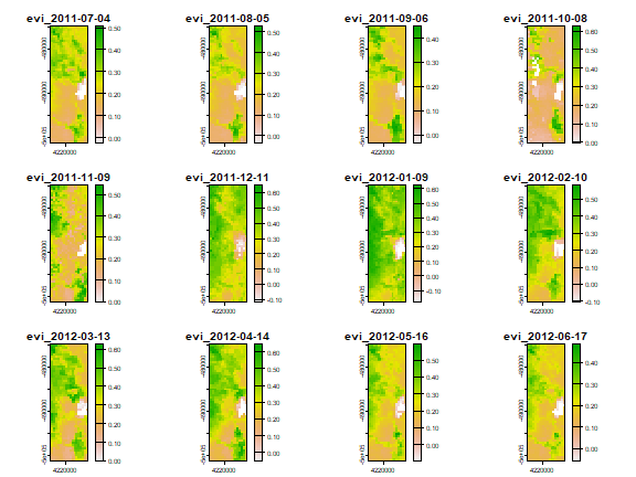
To have a quick look at spatio-temporal patterns in EVI we plot roughly 1 observation for each month. We are using 8-day interval data, so we use every fourth layer.
k <- seq(1, nlyr(evi), 4)
k
##  [1]  1  5  9 13 17 21 25 29 33 37 41 45
plot(evi[[k]])
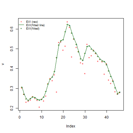
Next we use the luna::filterVI function for gap-filling/smoothing
and save the data to disk for future use. Our goal is to fit the upper
envelope of the time series values without excessive smoothing.
First for one grid cell:
v <- unlist(evi[200])
plot(v, pch = "*", col = "red")
s <- filterVI(v)
lines(s, col = "darkgreen")
points(s, pch="+", col = "darkgreen")
legend("topleft",
       legend = c("EVI (raw)", "EVI(fitted line)", "EVI(fitted)"),
       col = c("red","darkgreen", "darkgreen"),
       pch = c("*", NA, "+"), lty = c(NA, 1, NA),
       bty = "n", cex = 0.75)
There are number of parameters in the filterVI that affect the
quality of the EVI fitted values. You can vary parameters passed to
signal::sgolayfilt such as p (filter order) and n (filter
length). The optimal value can vary by region, so it can be useful to to
try different values.
And now we apply the filterVI function to all grid cells, using
terra::app.
# output direcotry
compdir <- file.path(datadir, "composite")
dir.create(compdir, recursive = TRUE, showWarnings = FALSE)
# run model and save output
fn <- file.path(compdir, paste0("/filter_evi_", year, ".tif"))
fevi <- app(evi, filterVI, filename = fn, overwrite=TRUE, wopt = list(names = names(evi)))
fn <- file.path(compdir, paste0("/filter_ndfi_", year, ".tif"))
fndfi <- app(ndfi, filterVI, filename=fn, overwrite =TRUE, wopt = list(names = names(ndfi)))
# also save the files used
saveRDS(evifiles, paste0(compdir, "/files_", year, "_evi.rds"))
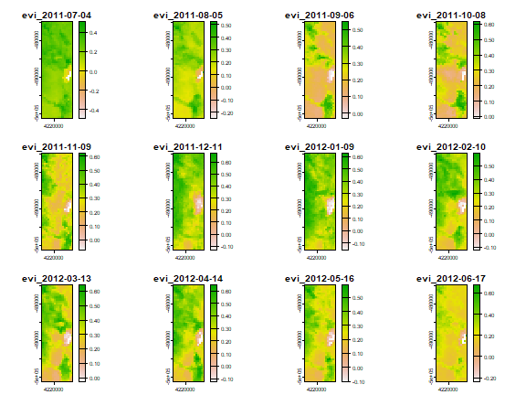
We can now plot the smoothed EVI. We use the same dates (one for each month) as above.
plot(fevi[[k]])
Rice mapping
Now we use the smooth time-series of remote sensing data for rice mapping. A number of algorithms have been developed that use such data to identify rice fields. The algorithms use multiple indices to detect different characteristics of the rice throughout the growing season namely: flooding and transplanting, heading (flowering) and harvest. For example, an important characteristics of flooded rice production is the presence of a water layer in the fields. Detecting water with remote sensing is relatively easy, and this is made use of in algorithms that focus on rice specifically.
Here we use the PhenoRice algorithm Boschetti et al. 2017 as implemnted in the R package phenorice.
We need a number of parameters representing the local rice growing conditions to apply the PhenoRice model. While we have some knowledge of the study area (growing season), we can examine EVI and NDFI time series profiles for finding other parameters (details later). In this case we have already estimated parameter values.
# create random locations to test the rice detection method
set.seed(4)
cells <- sample(ncell(evi), 200)
xy <- xyFromCell(evi, cells)
s <- vect(xy, crs=crs(evi))
# extract time series
ts_evi <- extract(evi, s, drop = TRUE)[,-1]
ts_fevi <- extract(fevi, s, drop = TRUE)[,-1]
ts_fndfi <- extract(fndfi, s, drop = TRUE)[,-1]
# Let's plot one sample that we already know is rice
i <- 121
dates <- evifiles$date
plot(dates, ts_evi[i,], pch = 16, col = "red", cex = 0.8, ylim = c(0,0.7),
        ylab = "vegetation indices", xlab = "dates",
        main = paste0("location_",i))
# smoothed values
lines(dates, ts_fevi[i,], col = "green")
lines(dates, ts_fndfi[i,], col = "blue")
legend("topleft", legend = c("EVI (raw)", "EVI", "NDFI"),
         pch = c(16, NA, NA), lty = c(NA, 1, 1),
         col = c("red", "green", "blue"), bty = "n", cex = 0.75)
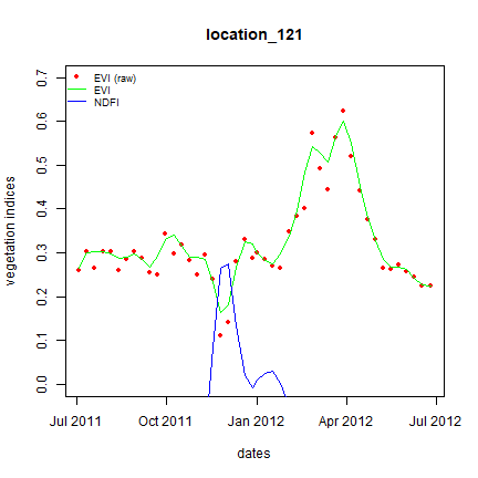
What we observe in the plot above is a short period with a high NDFI — this is indicative of a flooded area. Rice fields are typically flooded prior to transplanting. They will remain flooded, but as vegetation starts to grow and cover the water, the NDFI will go down. We see that here, as the the NDFI goes down with a strong increase in EVI. EVI reaches a plateau, and then drops again — this is a typical pattern for annual crops.
Below we plot phenology (EVI) of each sampling site at a time. We find
this is to be one of the best way to find phenorice parameters.
Notice the use of par(ask) to control plotting.
As you can see, NDFI is sensitive to the flooding event in the
transplanting phase of rice cultivation. After that EVI shows a regular
growth pattern of crops. But the NDFI signal is unique to transplanted
rice. Below we show how to apply the phenorice algorithm for
classifying point locations to separate rice and non-rice.
Below we show how to apply the phenorice algorithm for classifying
point locations to indentify rice areas. Phenorice needs a number of
parameters. There is a default set that you can get with
phenorice::getPars. Here we set all parameters manually after
inspecting the plots with EVI and NDFI. There may be better choices for
the parameters. At the same time, it’s better to keep the values
relaxed, e.g. if the maximum growing season duration is 150 - 180 days,
set the corresponding parameter around 200 days.
Important Note that we are dealing with MODIS 8-day product that makes 40 days difference equivalent to 5 units and so on).
library(phenorice)
p <- list()
p$evi_meanth <- 0.5 # threshold for annual mean EVI
p$evi_maxth <- 0.4  # threshold for maximum evi
p$evi_minth <- 0.3  # threshold for minimum evi
p$pos_start <- 20   # start of heading, after December
p$pos_end <- 40     # end of heading, not possible after April
p$vl1 <- 5          # the shortest vegetative growth length
p$vl2 <- 20         # the longest vegetative growth length
p$winfl <- 3        # period for flooding around min EVI
p$minndfi <- -0.1   # threshold for ndfi
p$windecr <- 15     # period after EVI maximum
p$decr <- 0.4      # fraction decrease of EVI before and after EVI maximum for EVI change ratecheck
p$tl1 <- 8          # shortest total growing length
p$tl2 <- 30         # the longest total growing length
p$lst_th <- 15      # the minimum temperature for planting
Now we can use ‘phenorice’ for our sample of cells to find the cells that have rice.
rice <- matrix(nrow=nrow(ts_fevi), ncol=5)
colnames(rice) <- c("start", "peak", "head", "flower", "mature")
ts_fevi <- as.matrix(ts_fevi)
ts_fndfi <- as.matrix(ts_fndfi)
for(i in 1:nrow(ts_fevi)){
  rice[i, ] <- phenorice(evi = ts_fevi[i,], ndfi = ts_fndfi[i,], p)
}
# output
head(rice)
##      start peak head flower mature
## [1,]     0    0  0.0      0      0
## [2,]     0    0  0.0      0      0
## [3,]    23   38 37.5     39     42
## [4,]    16   22 22.0     22     25
## [5,]    16   23 22.5     23     25
## [6,]    27   35 34.5     35     37
#ricedates <- dates[rice]
The phenorice algorithm not only identifies grid cells as rice or
not, it also returns five important dates in the rice growing season —
season start, peak greenness, flowering, heading and season end.
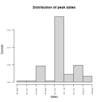
We can look at the distribution of values.
# Only keep records that has been detected as rice
s <- rowSums(rice, na.rm=TRUE) > 0
peak <- rice[s,1]
# distribution of peak
pdates <- as.Date(dates[peak])
hist(pdates, main = "Distribution of peak dates", xlab = "dates",
     breaks = "months", las = 2, cex.axis = 0.5)
## save phenology and rice information for future use
ricepheno <- list(ts_evi, ts_fevi, ts_fndfi, dates, rice)
names(ricepheno) <- c("evi_raw", "evi_fit", "ndfi", "dates", "phenorice")
saveRDS(ricepheno, paste0(compdir, "/ricepheno_", year, "_samples.rds"))
The ‘phenorice’ model can also be applied to the entire regions, with the evi and ndfi raster datasets.
# save result to a file
phenoraster <- file.path(compdir, paste0("/phenorice_", year, ".tif"))
x <- sds(fevi, fndfi)
phenomatrix <- function(x, y, p) {
  sapply(1:nrow(x), \(i) phenorice(x[i,], y[i,], p=p)) |> t()
}
r <- lapp(x, phenomatrix, filename=phenoraster, overwrite = TRUE, p=p,
         wopt = list(names = paste0(c("start", "peak", "head", "flower", "mature"),"_",year)))
plot(r)
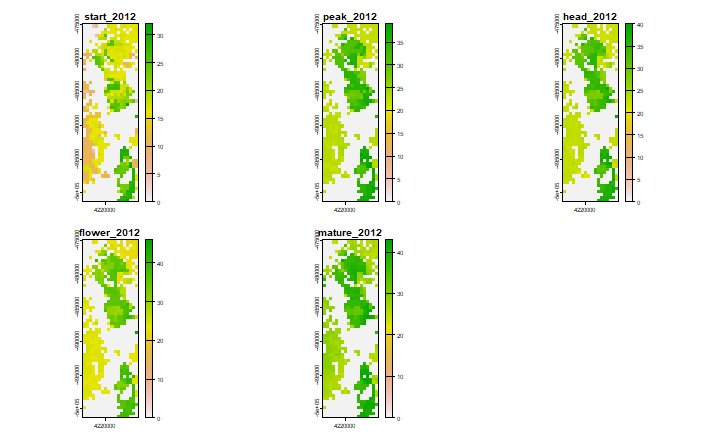
phenorice appears to work quite well in different environments. The great advantage is that you do need ground-truth data to train a supervised classification model with. However, these data should still be useful to evaluate the quality of the prediction in a particular region (and with a particular set of parameter values). It should be useful to have some data on the total rice area with regions; to help calibrate the model (by changing the parameters).
The additional benefit of the model is that it provides phenological stages. The algorithm could be adjusted to extract these stages for other crops as well (after detecting them with supervised classification).
We have found that “end of season” is the most difficult stage to accurately estimate. The algorithm tests for rate of change of evi after the peak that may be hard to detect for places with cloud cover during the later stage of the season.
Getting the season start dates can also be difficult. We have often
found that the start of the season is too early leading to unusually
long growing season. Peak, flowering and heading happen at close
interval and we find phenorice estimates to be reliable.