Yield Prediction

Introduction

In the previous chapters we have worked on identifying rice area, and the computations of vegetation metrics to predict rice yield. In this chapter we explore that relationship. The goal is to later use it to create an insurance product.

Yield data

We use a pre-prepared dataset with rice yield data that was collected through a farm survey. The numbers are based on the recollection of the farmers.

library(agrodata)
d <- data_rice("yield")
head(d, n=3)
##                 region     zone fid year    y
## 1401 Ndungu Irr Scheme Ndungu N   4 2003   40
## 1403 Ndungu Irr Scheme Ndungu N   4 2005 1296
## 1404 Ndungu Irr Scheme Ndungu N   4 2006 1296

We have rice yield, for individual farmers (“fid”) by year.

The number of farmers is

length(unique(d$fid))
## [1] 309

There are no missing values in this data set, so we can tabulate the number of observations by year like this:

table(d$year)
##
## 2003 2004 2005 2006 2007 2008 2009 2010 2011 2012
##   78   91  116  117  140  181  232  277  299  303

Farmers are grouped in zones

unique(d$zone)
##  [1] "Ndungu N"          "Ndungu S"          "Maore N"
##  [4] "Maore SE"          "Maore SW"          "Ndungu E"
##  [7] "Ndungu W"          "Sounthern Plain N" "Sounthern Plain S"
## [10] "Sounthern Plain W"

We can look at the distribution of rice yield values (they are expressed in kg/ha)

boxplot(d$y)

Some of the crop yields are extremely low. Here are the lowest 40 observations

sort(d$y)[1:40]
##  [1]   0.00000   0.00000   0.00000   0.00000   0.00000   0.00000   0.00000
##  [8]   0.00000   0.00000   0.00000   0.00000   0.00000   0.00000   0.00000
## [15]   0.00000   0.00000   0.00000   0.00000   0.00000   0.00000   0.00000
## [22]   0.00000   0.00000   0.00000   0.00000   0.00000   4.00000  40.00000
## [29]  40.00000  40.00000  48.00000  66.66667  66.66667  66.66667  70.00000
## [36]  80.00000  80.00000  80.00000  80.00000 100.00000

We may want to check if these are reasonable; or perhaps errors?

Aggregation

Regression models between yield and vegetation metrics may work better if we use average data for zones, rather than for individual farmers or fields; and that is what we do here.

Also, instead of the average yield, we could consider using the yield deviation, that is the difference between the yield in a given year (for a farmer or for a zone) and the expected yield.

The expected yield would be the long term average (mean or median) yield. The median could be a good choice. If there are outliers, it may better represents a “typical” (expected) yield. A benefit of this approach could be that it accounts for inherent differences between zones. That is some zones will have higher average yields that others; but they may be very similar in relative terms. We could also do this for the vegetation metrics.

So let’s create these aggregated variables for zones.

First the average yield for each zone/year combination:

yzt <- aggregate(d$y, d[, c("zone", "year")], median, na.rm=TRUE)
colnames(yzt)[3] = "y_zt"
head(yzt, 3)
##       zone year y_zt
## 1  Maore N 2003 1360
## 2 Maore SE 2003 1400
## 3 Maore SW 2003 1230

And the average yield for a zone (over years):

yz <- aggregate(d$y, d[, "zone", drop=FALSE], median, na.rm=TRUE)
colnames(yz)[2] = "y_z"
head(yz, 3)
##       zone  y_z
## 1  Maore N 1600
## 2 Maore SE 1440
## 3 Maore SW 1440

We can also use aggregate to compute the number of farmers per zone per year (note that this would not give the correct result if there are no missing values — as all records are counted).

n <- aggregate(d$fid, d[,c("zone", "year")], length)
colnames(n)[3] = "n"
head(n, 3)
##       zone year  n
## 1  Maore N 2003 13
## 2 Maore SE 2003  4
## 3 Maore SW 2003 10

Merge the zone level aggregates.

z <- merge(n, yzt)
z <- merge(z, yz)
head(z, 3)
##      zone year  n y_zt  y_z
## 1 Maore N 2003 13 1360 1600
## 2 Maore N 2004 18 1580 1600
## 3 Maore N 2005 22 1470 1600

Zone level relative yield can be compute like this:

z$y_dz <- z$y_zt / z$y_z
head(z, 3)
##      zone year  n y_zt  y_z    y_dz
## 1 Maore N 2003 13 1360 1600 0.85000
## 2 Maore N 2004 18 1580 1600 0.98750
## 3 Maore N 2005 22 1470 1600 0.91875

Here are the variables we now have (in data.frames d for farmer level and z for zone level)

variable	description
region	Region
zone	zone name
year	year
fid	farmer ID
y	reported yield for a farmer (i) in a year (t)
y_zt	mean zone yield in a year t
y_z	long term average zone yield

We save the zonal yield data for future use.

saveRDS(z, "zonal_rice_yield.rds")

We also merge the individual level data with the zone level data for use in the next chapter.

dz <- merge(d, z)
saveRDS(dz, "hh_rice_yield.rds")

Vegetation metrics

First read the pre-computed vegetation metrics.

idx <- data_rice("indices")
head(idx, n=3)
##          region    zone year     ndvi       evi       gpp       et       lai
## 1 Northern_zone Maore N 2003 1.420657 0.8657794 -696.7520 16.15727  39.73491
## 2 Northern_zone Maore N 2004 3.131069 1.9807431  630.2755 13.13894 115.83244
## 3 Northern_zone Maore N 2005 2.469837 1.9425927 -266.2523 24.80350 -53.02961
##       rain
## 1 689.2841
## 2 629.2459
## 3 543.0463

We have 5 different metrics computed for the growing season from MODIS data. They are all aggregated by zone.

variable	description
region	Region
zone	zone name
year	year
ndvi	ndvi index
evi index	evi
gpp	Gross Primary Productivity index
et	evapo-transpiration index
lai	leaf area index

The values have been transformed, and some may look a little odd (for example, they can be negative) — we are not going into these details here; let’s just accept them as they are.

We can merge the zonal yield and satellite index data.

z <- merge(z, idx[,-1])
head(z, 3)
##      zone year  n y_zt  y_z    y_dz     ndvi       evi       gpp       et
## 1 Maore N 2003 13 1360 1600 0.85000 1.420657 0.8657794 -696.7520 16.15727
## 2 Maore N 2004 18 1580 1600 0.98750 3.131069 1.9807431  630.2755 13.13894
## 3 Maore N 2005 22 1470 1600 0.91875 2.469837 1.9425927 -266.2523 24.80350
##         lai     rain
## 1  39.73491 689.2841
## 2 115.83244 629.2459
## 3 -53.02961 543.0463

Explore

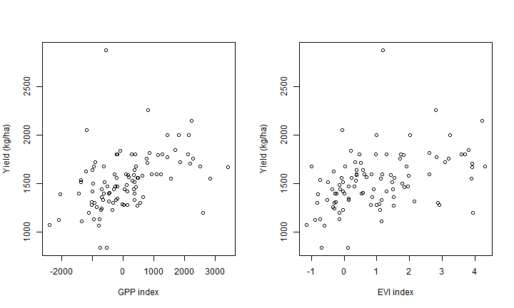
Let’s do a quick exploration of the combined data to see if we seen any association. Here are the correlation coefficients:

cr <- cor(z[,-c(1:3, 5)])
cr[,1:2]
##             y_zt         y_dz
## y_zt  1.00000000  0.892855126
## y_dz  0.89285513  1.000000000
## ndvi  0.40445628  0.379001496
## evi   0.41859193  0.389936563
## gpp   0.43046794  0.404100931
## et    0.27167524  0.254701878
## lai  -0.01201251 -0.036259112
## rain  0.02558946  0.002945276

These suggest that we the strongest relationships are between y_zt and gpp and evi, and also with ndvi.

Let’s plot the first two.

par(mfrow=c(1,2))
plot(z$gpp, z$y_zt, xlab="GPP index", ylab="Yield (kg/ha)")
plot(z$evi, z$y_zt, xlab="EVI index", ylab="Yield (kg/ha)")

Regression

Now on the the creation of regression models. There are many differnt models that could be formulated. We try a few, and compare them. Feel free to try other models.

First two single variable models. First zonal yield as a function of the gpp index.

m1 <- lm (y_zt ~ gpp, data=z)
cf <- coefficients(m1)
cf
##  (Intercept)          gpp
## 1516.4412306    0.1106993
plot(y_zt ~ gpp, data=z)
abline(m1, col="red")

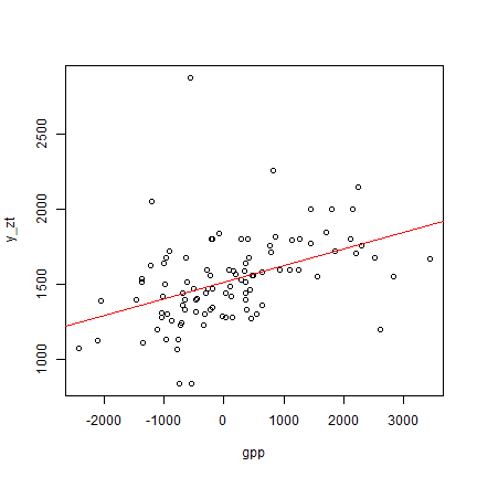
summary(m1)
##
## Call:
## lm(formula = y_zt ~ gpp, data = z)
##
## Residuals:
##     Min      1Q  Median      3Q     Max
## -617.33 -157.15  -18.93  115.10 1424.88
##
## Coefficients:
##              Estimate Std. Error t value Pr(>|t|)
## (Intercept) 1.516e+03  2.665e+01  56.904  < 2e-16 ***
## gpp         1.107e-01  2.345e-02   4.721 7.81e-06 ***
## ---
## Signif. codes:  0 '***' 0.001 '**' 0.01 '*' 0.05 '.' 0.1 ' ' 1
##
## Residual standard error: 265.3 on 98 degrees of freedom
## Multiple R-squared:  0.1853, Adjusted R-squared:  0.177
## F-statistic: 22.29 on 1 and 98 DF,  p-value: 7.811e-06

Have a good look at what is returned by summary.

First it shows the model that we formulated. Then it shows the distribution of the “residuals”. That is the differences between the observed values for y_zt and what the model would predict (the red line). You can get the residuals with residuals(m1).

Below that, the regression coefficients (under “Estimate”) are shown. There is an intercept of 1516.4 (that is the prediction when gpp=0), and a slope for gpp of 0.111. The good news is that the slope is positive (we expect that a higher gpp index is associated with higher yields). You can get the coefficients with coefficients(m1)

The standard error for each estimated coefficient is also shown. The t value is used to compute statistical signifiance. The p-values (the probabiliy to find, by chance, a t value that is higher then the ones we found) are very low and the coefficients are highly significant. In this context this means that is very unlikely that they are actually zero (no intercept, or no effect of evi).

Let’s try another model: zonal yield as a function of the evi index.

m2 <- lm (y_zt ~ evi, data=z)
summary(m2)
##
## Call:
## lm(formula = y_zt ~ evi, data = z)
##
## Residuals:
##     Min      1Q  Median      3Q     Max
## -607.49 -141.87   -4.27  126.25 1337.32
##
## Coefficients:
##             Estimate Std. Error t value Pr(>|t|)
## (Intercept)  1437.86      33.22  43.277  < 2e-16 ***
## evi            88.46      19.39   4.563 1.46e-05 ***
## ---
## Signif. codes:  0 '***' 0.001 '**' 0.01 '*' 0.05 '.' 0.1 ' ' 1
##
## Residual standard error: 267 on 98 degrees of freedom
## Multiple R-squared:  0.1752, Adjusted R-squared:  0.1668
## F-statistic: 20.82 on 1 and 98 DF,  p-value: 1.464e-05

The diagnistics for both models (as shown by summary) are very similar. Highly statistically significant, but a low R^2. Although p-values have information, we do not care that much about the significance — we are not testing a hypothesis. We do care about the R^2 as that is a measure of how good the regression model fits the data; and for simple models also a good indicator of how good it can make predictions.

Now to more complex (just a little) models. We can make a multiple regression model that explains y_zt from both gpp and evi.

m3 <- lm (y_zt ~ gpp + evi, data=z)
summary(m3)
##
## Call:
## lm(formula = y_zt ~ gpp + evi, data = z)
##
## Residuals:
##     Min      1Q  Median      3Q     Max
## -620.49 -146.08  -11.51  105.40 1390.32
##
## Coefficients:
##              Estimate Std. Error t value Pr(>|t|)
## (Intercept) 1.478e+03  4.131e+01  35.790   <2e-16 ***
## gpp         6.867e-02  4.211e-02   1.631    0.106
## evi         4.154e+01  3.461e+01   1.200    0.233
## ---
## Signif. codes:  0 '***' 0.001 '**' 0.01 '*' 0.05 '.' 0.1 ' ' 1
##
## Residual standard error: 264.8 on 97 degrees of freedom
## Multiple R-squared:  0.1972, Adjusted R-squared:  0.1807
## F-statistic: 11.92 on 2 and 97 DF,  p-value: 2.359e-05

We can add quadratic or interaction terms. Here we use a quadractic term for gpp. There is also a “zone” effect.

m4 <- lm (y_zt ~ gpp + evi +I(gpp^2) + zone, data=z)
summary(m4)
##
## Call:
## lm(formula = y_zt ~ gpp + evi + I(gpp^2) + zone, data = z)
##
## Residuals:
##     Min      1Q  Median      3Q     Max
## -573.13 -104.25    9.65   97.45 1316.10
##
## Coefficients:
##                         Estimate Std. Error t value Pr(>|t|)
## (Intercept)            1.390e+03  1.057e+02  13.141   <2e-16 ***
## gpp                    6.311e-02  4.359e-02   1.448   0.1513
## evi                    6.437e+01  4.339e+01   1.484   0.1415
## I(gpp^2)              -1.212e-05  1.541e-05  -0.787   0.4335
## zoneMaore SE           4.805e+01  1.173e+02   0.410   0.6831
## zoneMaore SW          -9.987e+01  1.155e+02  -0.865   0.3896
## zoneNdungu E           2.158e+02  1.278e+02   1.688   0.0949 .
## zoneNdungu N           2.975e+02  1.161e+02   2.562   0.0121 *
## zoneNdungu S           6.102e+01  1.204e+02   0.507   0.6134
## zoneNdungu W           1.367e+02  1.138e+02   1.201   0.2330
## zoneSounthern Plain N  2.750e+01  1.299e+02   0.212   0.8328
## zoneSounthern Plain S  4.883e+01  1.280e+02   0.381   0.7038
## zoneSounthern Plain W  8.300e+01  1.274e+02   0.651   0.5165
## ---
## Signif. codes:  0 '***' 0.001 '**' 0.01 '*' 0.05 '.' 0.1 ' ' 1
##
## Residual standard error: 253.9 on 87 degrees of freedom
## Multiple R-squared:  0.3378, Adjusted R-squared:  0.2464
## F-statistic: 3.698 on 12 and 87 DF,  p-value: 0.0001642

The “zone” paramter, allows for each zone to have its own intercept. Note that the R^2 is higher now, but that only the base intercept is highly significant.

We can also something entirely different, such as Random Forest

library(randomForest)
rf <- randomForest(y_zt ~ gpp+evi+ndvi+gpp+et, data=z)
rf
##
## Call:
##  randomForest(formula = y_zt ~ gpp + evi + ndvi + gpp + et, data = z)
##                Type of random forest: regression
##                      Number of trees: 500
## No. of variables tried at each split: 1
##
##           Mean of squared residuals: 73715.23
##                     % Var explained: 12.96

We see that the fit of the Random Forest model is not great. There is no magic machine learning here. Apparently there are not complex interactions to discover in this dataset.

Model comarpison

We have made four models. Which one is the best? We can compare R^2, adjusted R^2 and AIC.

models <- list(m1, m2, m3, m4)
r2 <- sapply(models, function(i) round(summary(i)$r.squared,  2))
ar2 <- sapply(models, function(i) round(summary(i)$adj.r.squared, 2))
aic <- sapply(models, AIC)
r <- rbind(r2=r2, ar2=ar2, aic=round(aic, 2))
colnames(r) <- c("m1", "m2", "m3", "m4")
r
##          m1      m2      m3      m4
## r2     0.19    0.18    0.20    0.34
## ar2    0.18    0.17    0.18    0.25
## aic 1403.97 1405.20 1404.50 1405.25

The R^2 values are between 0.18 and 0.34. The problem with using R^2 on the model training data is that it will always get higher as you add parameters to the model. It is thus not surprising that the most complex model has the highest R^2.

The Adjusted-R^2 corrects for this problem — for each additional parameter in the model, the R^2 is penalized. Thus for it to go up, the benefit of the new variable must outweight the cost (because of this you can even get negative values — wich seem very odd for a squared quantity). We see that the adjusted R^2 is much lower than the R^2 for thet complex model (m4) has a much reduced adjfit whereas the simpler .

AIC is a measure that can be used to find the most parsimonious model. That is, the simplest model that described the data well.

Cross-validation

We need a function that returns Root Mean Squared Error (or another statistic of interest)

rmse <- function(observed, predicted){
  i <- observed < 1500
  error <- observed[i] - predicted[i]
  sqrt(mean(error^2))
}

Now set up the “k-folds” and the output structure.

library(agro)
k <- 5
set.seed(123)
f <- agro::make_groups(z, k)
result <- matrix(nrow=k, ncol=5)
colnames(result) <- c("m1", "m2", "m3", "m4", "rf")

And run the actual cross-validation.

for (i in 1:k) {
  train <- z[f!=i, ]
  test  <- z[f==i, ]
  cm1 <- lm (y_zt ~ gpp, data=train)
  cm2 <- lm (y_zt ~ evi, data=train)
  cm3 <- lm (y_zt ~ gpp + evi, data=train)
  cm4 <- lm (y_zt ~ gpp + evi +I(gpp^2) + zone, data=train)
  p <- predict(cm1, test)
  result[i,"m1"] <- rmse(test$y_zt, p)
  result[i,"m2"] <- rmse(test$y_zt, predict(cm2, test))
  result[i,"m3"] <- rmse(test$y_zt, predict(cm3, test))
  result[i,"m4"] <- rmse(test$y_zt, predict(cm4, test))
  crf <- randomForest(y_zt ~ gpp+evi+ndvi+gpp+et, data=train)
  result[i,"rf"] <- rmse(test$y_zt, predict(crf, test))
}
colMeans(result)
##       m1       m2       m3       m4       rf
## 213.6315 229.9579 225.4810 271.2868 243.1905

Note that m1 comes out as the best model (lowest RMSE), but m2 and m3 are very close. Of these three models, we should probably prefer m1 for the contract design.

m4 looked the best, but the cross-validation results now suggests that m4 is overfitted and should not be used.

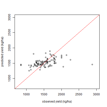
We can make a plot of osberved vs predicted values for the models. Here for m1.

plot(z$y_zt, predict(m1), xlim=c(750, 3000), ylim=c(750, 3000), xlab="observed yield (kg/ha)", ylab="predicted yield (kg/ha)")
abline(a=0,b=1, col="red")

Saving the models

mods <- list(m1=m1, m2=m2, m3=m3, m4=m4)
saveRDS(mods, "rice_models.rds")