Computing vegetation metrics

Introduction

In the previous section, we used the phenorice algorithm to detect rice fields and calculate important phenological dates.

We also used that information to calculate different vegetation indices from the gap-filled time series data. Next we show how to use the phenology information to compute metrics that can be indicators of yield variability. We assume that the sum of the vegetation index during the growing is an indicator of the productivity. We will use the data generated for rice phenology detection.

Data

library(luna)
# set directories
datadir <- file.path(dirname(tempdir()), "agrins")
compdir <- file.path(datadir, "composite")
dir.create(compdir, recursive = TRUE, showWarnings = FALSE)
# rice phenology information
year <- 2012
ricepheno <- readRDS(paste0(compdir, "/ricepheno_",year,"_samples.rds"))
# we need the following three for this exercise
vi <- ricepheno[["evi_fit"]]
dates <- ricepheno[["dates"]]
rice <- ricepheno[["phenorice"]]

Metrics

To compute metrics, we aggregate the time series information between two dates by computing the “area under the curve” for a vegetation index.

You can choose the dates based on what works best for your purposes. For example, you can take the entire growing season (“full season”), or only up to the date that the vegetation index reaches its maximum value (“early season”); or from the peak to the end of the season (“late season”).

Before the aggregation, it may be helpful to remove the background signal, that is, we subtract the lowest value observed.

What do these metrics look like? Let’s find out with a single pixel time series.

# valid rice records
s <- which(rowSums(rice, na.rm=TRUE) > 0)
# let's consider one of them
p1 <- rice[s[1], ]
# peak
print(p1)
##  start   peak   head flower mature
##   23.0   38.0   37.5   39.0   42.0
peak <- p1[2]
start <- p1[1]
mature <- p1[5]
# corresponding fitted time series
v1 <- unlist(vi[s[1],])
# remove background signal
v1 <- v1 - min(v1)
# plots
plot(v1, type = "l", col = "darkgreen", ylim = c(min(v1), max(v1)*1.25),
      ylab = "EVI", xlab = "date", xaxt = "n", main = "EVI based index")
at <- seq(1, length(v1), 4)
labs <- months(dates[at])
axis(1, at = at, labels = substr(labs, 1,3), las = 2)
# vegetative
polygon(x=c(start,start:peak,peak),
        y=c(0, v1[start:peak], 0),
        col="green")
# grain-filling
polygon(x=c(peak, peak:mature, mature),
        y=c(0, v1[peak:mature], 0), col="yellow")
# add full growing season
polygon(x=c(start,start:mature, mature),
        y=c(0, v1[start:mature], 0),
        col="red", density=10)
# add legend
legend("topleft", legend=c("vegetative","grain","full"), fill=c("green", "yellow", "red"), density=c(NA, NA, 20), bty="n", border="black")

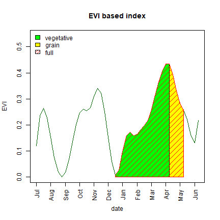
To compute the area under curve we can use numerical integration. As we use data at constant intervals (8 days) we simply sum the vegetation index values within the date window. Next we compute temporal aggregates for three intervals—vegetative, grain-filling and full season.

# vegetative growth
i1 <- sum(v1[start:peak], na.rm = TRUE)
# reproductive
i2 <- sum(v1[peak:mature], na.rm = TRUE)
# full season
i3 <- sum(v1[start:mature], na.rm = TRUE)
ind <- c(i1, i2, i3)
names(ind) <- paste0("idx_evi_", c("v","g","f"))

These metrics can be used to predict crop yield. We show the process for a single year for a single pixel that can be extended for multiple years and also to other type of indices, such as GPP, ET, LAI/FPAR.

As we don’t generally know which metrics will work for what conditions or crops. It is advisable to test multiple metrics to find the best ones for yield prediction.

Likewise there is no consensus on the ‘best’ index or how to preform the temporal aggregation. In the previous chapter, we briefly discussed that among all the phenology information, peak can be measure most reliably. Therefore it may make sense use a number of days around the peak, for example, 30 days at each side. In that case we would replace start with peak-4 and mature with peak+4.

Next we expand this calculation using a function that can be used for either a set of pixels for an entire raster.

getAUC <- function(v, peak, start, mature){
  ind <- c(NA, NA, NA)
  peak <- as.vector(peak)
  start <- as.vector(start)
  mature <- as.vector(mature)
  # check both NA and NaN
  if (sum(is.na(v)) > 5) return(ind)
  if(is.na(sum(peak, start, mature))) return(ind)
  # vegetative growth
  i1 <- sum(v[start:peak], na.rm = TRUE)
  # reproductive
  i2 <- sum(v[peak:mature], na.rm = TRUE)
  # full season
  i3 <- sum(v[start:mature], na.rm = TRUE)
  ind <- c(i1,i2,i3)
  return(ind)
}
# apply to single pixel
a1 <- getAUC(v1, peak = 37, start = 32, mature = 42)
names(a1) <- paste0("idx_evi_", c("v","g","f"))
# compare the value with the earlier index calculated based phenorice derived dates
ind
## idx_evi_v idx_evi_g idx_evi_f
##  3.590148  1.695379  4.851318
a1
## idx_evi_v idx_evi_g idx_evi_f
##  1.992271  2.129552  3.687650

Now we apply this function to the raster data

library(terra)
## terra 1.7.36
year <- 2012
fevi <- rast(file.path(compdir, paste0("/filter_evi_", year, ".tif")))
phenoraster <- rast(file.path(compdir, paste0("/phenorice_", year, ".tif")))
# for simplicity we assume average phenology dates for the region
ar <- app(fevi, getAUC, peak = 37, start = 30, mature = 43)
names(ar) <- paste0("idx_evi_", c("v","g","f"))
# but we could replace this with something like this
#ff <- c(s+3, p+3, m+3, ar)
#ar = app(ff, function(x) c(sum(x[x[1]:x[2]], na.rm=T),
#                            sum(x[x[2]:x[3]], na.rm=T),
#                            sum(x[x[1]:x[3]], na.rm=T)) )
# mask metrics by rice growing pixels
maskfun <- function(x){
  x <- sum(x, na.rm = TRUE)
  x[is.na(x)] <- 0
  x[x==0] <- NA
  x[!is.na(x)] <- 1
  return(x)
}
# apply rice mask
ricemask <- app(phenoraster, fun = maskfun)
arm <- mask(ar, ricemask)

Aggregate

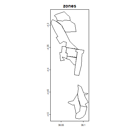
Once we have the metrics values estimated for the entire study region, we can find the metrics for an individual farmer or spatial aggregate over the zone. The following example show how to spatially aggregate the metrics over the insurance zones.

# get insurance zones
z <- agrodata::data_rice("zones")
plot(z, main = "zones")

# transform z to the crs of arm
z <- project(z, crs(arm))
# extract zone-level metrics and add the id
mz <- extract(arm, z, fun=mean, na.rm=TRUE)
# merge with zones
values(z) <- cbind(as.data.frame(z), mz)

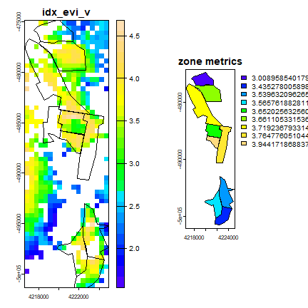
Let’s plot the spatial distribution of zone level metrics values after removing the ones with few (< 10) pixels/plots.

# remove zones with few pixels
n <- extract(ricemask, z, fun=sum, na.rm=TRUE)
n <- which(n[,2] > 10)
mzv <- z[n,]
# We only plot the first metrics ~ AUC under vegetative growth
par(mfrow = c(1,2))
plot(arm[["idx_evi_v"]], main = "idx_evi_v", col=topo.colors(25))
plot(z, add = T)
plot(mzv, "idx_evi_v", main = "zone metrics", col=topo.colors(25))

In the first 4 chapters we showed you how to compute metrics for yield index starting with downloading on MODIS data. The exercises use one year of MODIS EVI data. These steps can be applied for multiple years of data to create long term record of the metrics and also incorporate other MODIS products (such as GPP, ET).

In the next chapter, we examine the performance of different pre-computed metrics for yield estimations.